Real world data can contain missing values due to human error in collection, storage issues, faulty sensors, etc., If a supervised learning datapoint is missing its output value - e.g., if a classification datapoint is missing its label - there can be little we can do to salvage the datapoint, and usually such a corrupted datapoint is thrown away. Likewise, if a large number of the values of an input are missing the data is best discarded. However a datapoint whose input is missing just a handful of input (feature) values can be salvaged, and such points should be salvaged since data is often a scarce resource. Because machine learning models take in only numerical valued objects, in order for us to be able to use a datapoint with missing entries in training any machine learning model we must fill in missing input features with numerical values (this is often called imputing). But what values should we set missing entries too?

Imputing using the mean¶

Suppose we have a set of $P$ inputs, each of which is $N$ dimensional, and say that the $j^{th}$ point has is missing its $n^{th}$ input feature value. In other words, the value $x_{j,n}$ is missing from our input data. A reasonable value to fill for this missing entry is simply the average of the dataset along this dimension, since this can roughly be considered the 'standard' value of our input along this dimension. If in particular we use the mean $\mu_n$ of our input along this dimension (ignoring our missing entry $x_{j,n}$) we set $x_{j,n} = \mu_n$ where

\begin{equation} \mu_n = \frac{1}{P-1} \sum_{\underset{p \neq j}{j=1}}^P x_{p,n}. \end{equation}

This is often called mean-imputation.

Notice how, in mean-imputing $x_{p,n}$, that the mean value of the entire $n^{th}$ feature of the input with the inputed value does not change. We can see this by simply computing the mean of the new $n^{th}$ input dimension as

\begin{equation} \frac{1}{P} \sum_{p=1}^P x_{p,n} = \frac{1}{P} \sum_{\underset{p \neq j}{j=1}}^P x_{p,n} + \frac{1}{P} x_{j,n} = \frac{P - 1}{P} \frac{1}{P-1} \sum_{\underset{p \neq j}{j=1}}^Px_{p,n} + \frac{1}{P} x_{j,n} = \frac{P - 1}{P} \mu_n + \frac{1}{P} \mu_n = \mu_n. \end{equation}

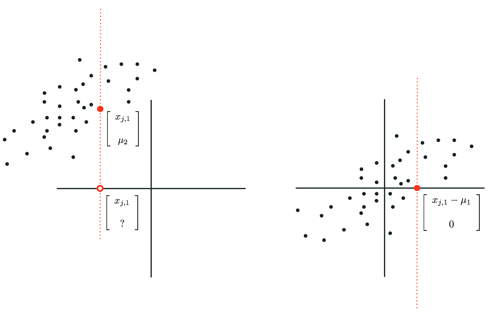
Also notice that if we impute missing values of a dataset using the mean along each input dimension that if we then standard normalize this dataset, all values imputed with the mean become exactly zero. Because the mean of an input feature that has been imputed with mean values does not change (as shown above), when we mean-center the dataset (the first step in standard normalization) by subtracting the mean of this input dimension the resulting value becomes exactly zero (this is illustrated in the figure below for a simple case where $N = 2$). Any model weight touching such a mean-imputed entry is then comopletely nullified numerically. In other words, in training any mean-imputed value will not directly contribute to the tuning of its associated feature weight (provided the input has been standard normalized). This is very desireable given that such values were missing to begin with.

More generally if our input is missing multiple entries along this dimension we can just as reasonably replace each one with the mean along the $n^{th}$ feature, where in computing this mean we once again exclude missing values. Again one can see that with these imputed values the mean along this dimension does not change.