code

share


As we have seen with logistic regression we treat classification as a particular form of nonlinear regression (employing - with the choice of label values $y_p \in \left\{-1,+1\right\}$ - a tanh nonlinearity). This results in the learning of a proper nonlinear regressor, and a corresponding linear decision boundary
\begin{equation} \mathring{\mathbf{x}}_{\,}^{T}\mathbf{w}^{\,}=0. \end{equation}
Instead of learning this decision boundary as a result of a nonlinear regression, the perceptron derivation described in this Section aims at determining this ideal lineary decision boundary directly. While we will see how this direct approach leads back to the Softmax cost function, and that practically speaking the perceptron and logistic regression often results in learning the same linear decision boundary, the perceptron's focus on learning the decision boundary directly provides a valuable new perspective on the process of two-class classification. In particular - as we will see here - the perceptron provides a simple geometric context for introducing the important concept of regularization (an idea we will see arise in various forms throughout the remainder of the text).
With two-class classification we have a training set of $P$ points $\left\{ \left(\mathbf{x}_{p},y_{p}\right)\right\} _{p=1}^{P}$ - where $y_p$'s take on just two label values from $\{-1, +1\}$ - consisting of two classes which we would like to learn how to distinguish between automatically. As we saw in our discussion of logistic regression, in the simplest instance our two classes of data are largely separated by a linear decision boundary with each class (largely) lying on either side. This decision boundary, written as
\begin{equation} \mathring{\mathbf{x}}^{T}\mathbf{w}^{\,} = 0, \end{equation}
is a point when the dimension of the input is $N=1$ (as we saw in e.g., Example 2 of the previous Section), a line when $N = 2$ (as we saw in e.g, Example 3 of the previous Section), and is more generally for arbitray $N$ a hyperplane defined in the input space of a dataset. This scenario can be best visualized in the case $N=2$, where we view the problem of classification 'from above' - showing the input of a dataset colored to denote class membership. The default coloring scheme we use here - matching the scheme used in the previous Section - is to color points with label $y_p = -1$ blue and $y_p = +1$ red. The linear decision boundary is here a line that best separates points from the $y_p = -1$ class from those of the $y_p = +1$ class, as shown figuratively in the panels below.
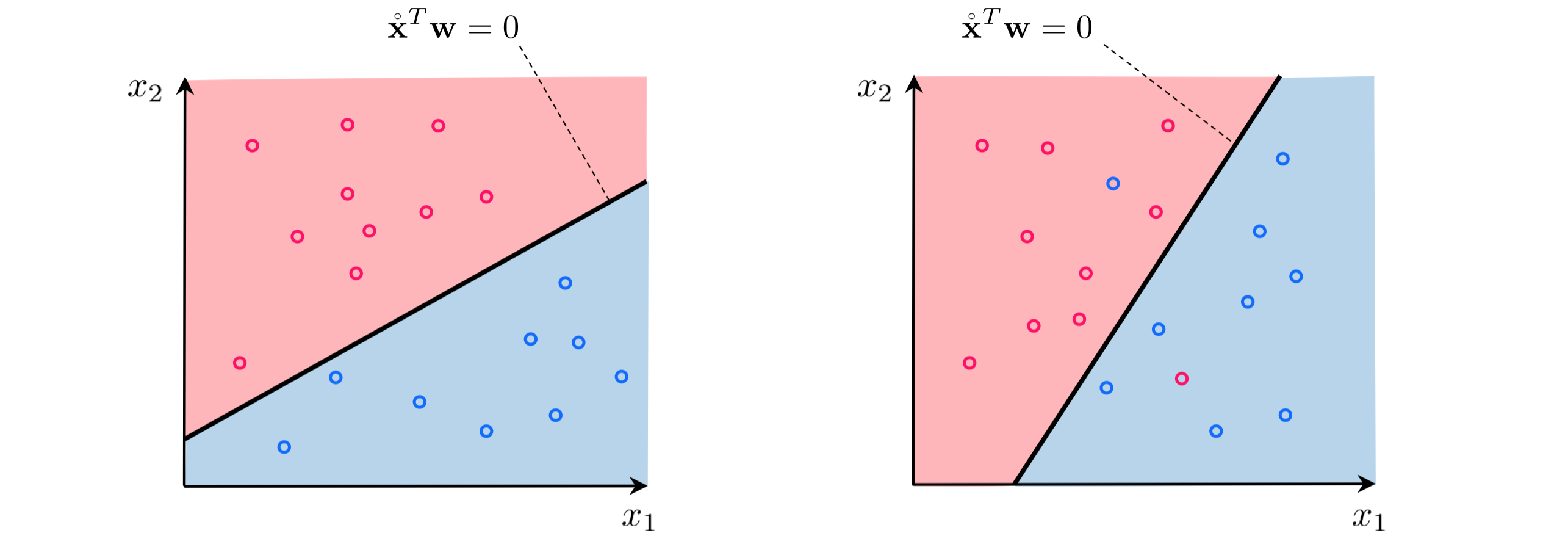
A linear decision boundary cuts the input space into two half-spaces, one lying 'above' the hyperplane where $\mathring{\mathbf{x}}^{T}\mathbf{w}^{\,} > 0$ and one lying 'below' it where $\mathring{\mathbf{x}}^{T}\mathbf{w}^{\,} < 0$. Notice then, as depicted visually in the figure above, that a proper set of weights $\mathbf{w}$ define a linear decision boundary that separates a two-class dataset as well as possible with as many members of one class as possible lying above it, and likewise as many members as possible of the other class lying below it. Because we can always flip the orientation of an ideal hyperplane by multiplying it by $-1$ (or likewise because we can always swap our two label values) we can say more specifically that when the weights of a hyperplane are tuned properly members of the class $y_p = +1$ lie (mostly)'above' it, while members of the $y_p = -1$ class lie (mostly) 'below' it. In other words, our desired set of weights define a hyperplane where as often as possible we have that
\begin{equation} \begin{array} \ \mathring{\mathbf{x}}_{p}^T\mathbf{w}^{\,} >0 & \,\,\,\,\text{if} \,\,\, y_{p}=+1\\ \mathring{\mathbf{x}}_{p}^T\mathbf{w}^{\,} <0 & \,\,\,\,\text{if} \,\,\, y_{p}=-1. \end{array} \end{equation}
Because of our choice of label values we can consolidate the ideal conditions above into the single equation below
\begin{equation} -\overset{\,}{y}_{p}\mathring{\mathbf{x}}_{p}^T\mathbf{w}^{\,} <0. \end{equation}
Again we can do so specifically because we chose the label values $y_p \in \{-1,+1\}$. Likewise by taking the maximum of this quantity and zero we can then write this ideal condition, which states that a hyperplane correctly classifies the point $\mathbf{x}_{p}$, equivalently forming a point-wise cost
\begin{equation} g_p\left(\mathbf{w}\right) = \text{max}\left(0,\,-\overset{\,}{y}_{p}\mathring{\mathbf{x}}_{p}^T\mathbf{w}^{\,}\right)=0 \end{equation}
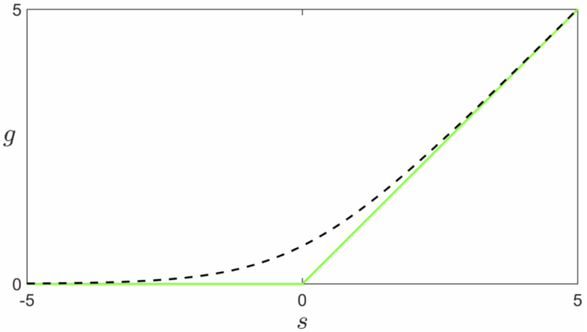
Note that the expression $\text{max}\left(0,-\overset{\,}{y}_{p}\mathring{\mathbf{x}}_{p}^T\mathbf{w}^{\,}\right)$ is always nonnegative, since it returns zero if $\mathbf{x}_{p}$ is classified correctly, and returns a positive value if the point is classified incorrectly. The functional form of this point-wise cost $\text{max}\left(0,\cdot\right)$ is called a rectified linear unit (see the Appendix of this text for a historical explination of this term). Because these point-wise costs are nonnegative and equal zero when our weights are tuned correctly, we can take their average over the entire dataset to form a proper cost function as
\begin{equation} g\left(\mathbf{w}\right)= \frac{1}{P}\sum_{p=1}^Pg_p\left(\mathbf{w}\right) = \frac{1}{P}\sum_{p=1}^P\text{max}\left(0,-\overset{\,}{y}_{p}\mathring{\mathbf{x}}_{p}^T\mathbf{w}^{\,}\right). \end{equation}
When minimized appropriately this cost function can be used to recover the ideal weights satisfying equations (3) - (5) as often as possible.
This cost function goes by many names such as the perceptron cost, the rectified linear unit cost (or ReLU cost for short), and the hinge cost (since when plotted a ReLU function looks like a hinge). This cost function is always convex but has only a single (discontinuous) derivative in each input dimension. This implies that we can only use zero and first order local optimization schemes (i.e., not Newton's method). Note that the perceptron cost always has a trivial solution at $\mathbf{w} = \mathbf{0}$, since indeed $g\left(\mathbf{0}\right) = 0$, thus one may need to take care in practice to avoid finding it (or a point too close to it) accidentally.
Learning and optimization go hand in hand, and as we know from the discussion above the ReLU function limits the number of optimization tools we can bring to bear for learning. It not only prohibits the use of Newton's method but forces us to be very careful about how we choose our steplength parameter $\alpha$ with gradient descent as well (as detailed in the example above). Here we describe a common approach to ameliorating this issue by introducing a smooth approximation to this cost function. This practical idea takes many forms depending on the cost function at play, but the general idea is this: when dealing with a cost function that has some deficit (insofar as local optimization is concerned) replace it with a smooth (or at least twice differentiable) cost function that closely matches it everywhere. If the approximation closely matches the true cost function then for the small amount of accuracy (we will after all be minimizing the approximation, not the true function itself) we significantly broaden the set of optimization tools we can use.
One popular way of doing this for the ReLU cost function is via the softmax function defined as
\begin{equation} \text{soft}\left(s_0,s_1,...,s_{C-1}\right) = \text{log}\left(e^{s_0} + e^{s_1} + \cdots + e^{s_{C-1}} \right) \end{equation}
where $s_0,\,s_1,\,...,s_{C-1}$ are any $C$ scalar vaules - which is a generic smooth approximation to the max function, i.e.,
\begin{equation} \text{soft}\left(s_0,s_1,...,s_{C-1}\right) \approx \text{max}\left(s_0,s_1,...,s_{C-1}\right) \end{equation}
To see why the softmax approximates the max function let us look at the simple case when $C = 2$.
Suppose momentarily that $s_{0}\leq s_{1}$, so that $\mbox{max}\left(s_{0},\,s_{1}\right)=s_{1}$. Therefore $\mbox{max}\left(s_{0},\,s_{1}\right)$ can be written as $\mbox{max}\left(s_{0},\,s_{1}\right)=s_{0}+\left(s_{1}-s_{0}\right)$, or equivalently as $\mbox{max}\left(s_{0},\,s_{1}\right)=\mbox{log}\left(e^{s_{0}}\right)+\mbox{log}\left(e^{s_{1}-s_{0}}\right)$. Written in this way we can see that $\mbox{log}\left(e^{s_{0}}\right)+\mbox{log}\left(1+e^{s_{1} s_{0}}\right)=\mbox{log}\left(e^{s_{0}}+e^{s_{1}}\right)=\mbox{soft}\left(s_{0},s_{1}\right)$ is always larger than $\mbox{max}\left(s_{0},\,s_{1}\right)$ but not by much, especially when $e^{s_{1}-s_{0}}\gg1$. Since the same argument can be made if $s_{0}\geq s_{1}$ we can say generally that $ $$\mbox{soft}\left(s_{0},s_{1}\right)\approx\mbox{max}\left(s_{0},s_{1}\right)$. The more general case follows similarly as well.
Returning to the ReLU perceptron cost function in equation (5), we replace the $p^{th}$ summand with its softmax approximation, making this our point-wise cost
\begin{equation} g_p\left(\mathbf{w}\right) = \text{soft}\left(0,-\overset{\,}{y}_{p}\mathring{\mathbf{x}}_{p}^T\mathbf{w}^{\,}\right)= \text{log}\left(e^{0} + e^{-\overset{\,}{y}_{p}\mathring{\mathbf{x}}_{p}^T\mathbf{w}^{\,}}\right) = \text{log}\left(1 + e^{-\overset{\,}{y}_{p}\mathring{\mathbf{x}}_{p}^T\mathbf{w}^{\,}}\right) \end{equation}
giving the overall cost function as
\begin{equation} g\left(\mathbf{w}\right)=\sum_{p=1}^P g_p\left(\mathbf{w}\right) = \underset{p=1}{\overset{P}{\sum}}\text{log}\left(1 + e^{-\overset{\,}{y}_{p}\mathring{\mathbf{x}}_{p}^T\mathbf{w}^{\,}}\right) \end{equation}
which is the Softmax cost we saw previously derived from the logistic regression perspective on two-class classification in the previous Section. This is why the cost is called Softmax, since it derives from the general softmax approximation to the max function.
Note that like the ReLU cost - as we already know - the Softmax cost is convex. However unlike the ReLU cost, the softmax has infinitely many derivatives and Newton's method can therefore be used to minimize it. Moreover, softmax does not have a trivial solution at zero like the ReLU cost does. Nonetheless, the fact that the Softmax cost so closely approximates the ReLU shows just how closely aligned - in the end - both logistic regression and the perceptron truly are. Practically speaking their differences lie in how well - for a particular dataset - one can optimize either one, along with (what is very often slight) differences in the quality of each cost function's learned decision boundary. Of course when the Softmax is employed from the perceptron perspective there is no qualitative difference between the perceptron and logistic regression at all.
Imagine that we have a dataset whose two classes can be perfectly separated by a hyperplane, and that we have chosen an appropriate cost function to minimize it in order to determine proper weights for our model. Imagine further that we are extremely lucky and our initialization $\mathbf{w}^0$ produces a linear decision boundary $\mathring{\mathbf{x}}_{\,}^T\mathbf{w}^{0} = 0$ with perfect sepearation. This means that - according to equation (4) - that for each of our $P$ points we have that
\begin{equation} -\overset{\,}{y}_{p}\mathring{\mathbf{x}}_{p}^T\mathbf{w}^{0} <0 \end{equation}
and likewise that the point-wise RelLU cost in equation (5) is zero for every point i.e., $g_p\left(\mathbf{w}^0\right) = \text{max}\left(0,\,-\overset{\,}{y}_{p}\mathring{\mathbf{x}}_{p}^T\mathbf{w}^{0}\right)=0$ and so the ReLU cost is exactly equal to zero
\begin{equation} g\left(\mathbf{w}^0\right) = \frac{1}{P}\sum_{p=1}^P\text{max}\left(0,-\overset{\,}{y}_{p}\mathring{\mathbf{x}}_{p}^T\mathbf{w}^{0}\right) = 0. \end{equation}
Since the ReLU cost value is already zero, its lowest value, this means that we would halt our local optimization immediately. For example, since the gradient of this cost is also zero at $\mathbf{w}^0$ (see Example 1 above where the form of this gradient was given) a gradient descent step would not move us from $\mathbf{w}^0$. However this will not happen if we instead employed the Softmax cost.
Since the quantity $-\overset{\,}{y}_{p}\mathring{\mathbf{x}}_{p}^T\mathbf{w}^{0} <0$ its negative exponential is larger than zero i.e., $e^{-\overset{\,}{y}_{p}\mathring{\mathbf{x}}_{p}^T\mathbf{w}^{0}} > 0$, which means that the softmax point-wise cost is also nonnegative $g_p\left(\mathbf{w}^0\right) = \text{log}\left(1 + e^{-\overset{\,}{y}_{p}\mathring{\mathbf{x}}_{p}^T\mathbf{w}^{0}}\right) > 0$ and hence too the Softmax cost is nonnegative as well
\begin{equation} g\left(\mathbf{w}^0\right)= \sum_{p=1}^P\text{log}\left(1 + e^{-\overset{\,}{y}_{p}\mathring{\mathbf{x}}_{p}^T\mathbf{w}^{0}}\right) > 0. \end{equation}
This means that we in applying any local optimization scheme like e.g., gradient descent we will indeed take steps away from $\mathbf{w}^0$ in order to drive the value of the Softmax cost lower and lower towards its minimum at zero. In fact - with data that is indeed linearly separable - the Softmax cost achieves this lower bound only when the magnitude of the weights grows to infinity. This is clear from the fact each individual term $\text{log}\left(1 + e^{-C}\right) = 0$ only as $C \longrightarrow \infty$. Indeed if we multiply our initialization $\mathbf{w}^0$ by any constant $C > 1$ we can decrease the value of any negative exponential involving one of our data points since $e^{-C} < 1$ and so
\begin{equation} e^{-\overset{\,}{y}_{p}\mathring{\mathbf{x}}_{p}^TC\mathbf{w}^{0}} = e^{-C}e^{-\overset{\,}{y}_{p}\mathring{\mathbf{x}}_{p}^T\mathbf{w}^{0}} < e^{-\overset{\,}{y}_{p}\mathring{\mathbf{x}}_{p}^T\mathbf{w}^{0}}. \end{equation}
This likewise decreases the Softmax cost as well with the minimum achieved only as $C \longrightarrow \infty$. Note however that regardless of the scalar $C > 1$ value involved the decision boundary defined by the initial weights $\mathring{\mathbf{x}}_{\,}^T\mathbf{w}^{0} = 0$ does not change location, since we still have that $C\,\mathring{\mathbf{x}}_{\,}^T\mathbf{w}^{0} = 0$ (indeed this is true for any non-zero scalar $C$). So even though the location of the separating hyperplane need not change, with the Softmax cost we still take more and more steps in minimization since (in the case of linearly separable data) its minimum lies off at infinity. This can cause severe numerical instability issues with local optimizaiton schemes that make large progress at each step - particularly Newton's method - since they will tend to rapidly diverge to infinity.
Notice: because the Softmax and Cross-Entropy costs are equivalent (as discussed in the previous Section), this issue equally presents itself when using the Cross-Entropy cost as well.
In applying Newton's method to minimize the Softmax over linearly separable data it is easily possible to run into numerical instability issues as the global minimum of the cost technically lies at infinity. Here we examine a simple instance of this behavior using the single input dataset shown in the previous Section. In this example we illustrate the progress of 5 Newton steps beginning at the point $\mathbf{w} = \begin{bmatrix} 1 \\ 1 \end{bmatrix}$. Within 5 steps we have reached a point providing a very good fit to the data (here we plot the $\text{tanh}\left(\cdot\right)$ fit using the logistic regressoion perspective on the Softmax cost), and one that is already quite large in magnitude (as can be seen in the right panel below). We can see here by the trajectory of the steps, which are traveling linearly towards the mininum out at $\begin{bmatrix} -\infty \\ \infty \end{bmatrix}$, that the location of the linear decision boundary (here a point) is not changing after the first step or two. In other words, after the first few steps we each subsequent step is simply multiplying its predecessor by a scalar value $C > 1$.

Notice that if we simply flip one of the labels - making this dataset not perfectly linearly separable - the corresponding cost function does not have a global minimum out at infinity, as illustrated in the contour plot below.

How can we prevent this potential problem when employing the Softmax or Cross-Entropy cost? One approach can be to employ our local optimization schemes more carefully by eg., taking fewer steps and / or halting a scheme if the magnitude of the weights grows larger than a large pre-defined constant (this is called early-stopping). Another approach is to control the magnitude of the weights during the optimization procedure itself. Both approaches are generally referred to in the jargon of machine learning as regularization strategies. The former strategy is straightfoward, requiring slight adjustments to the way we have typically employed local optimization, but the latter approach requires some further explanation which we now provide.
To control the magnitude of $\mathbf{w}$ means that we want to control the size of the $N+1$ individual weights it contains
\begin{equation} \mathbf{w} = \begin{bmatrix} w_0 \\ w_1 \\ \vdots \\ w_N \end{bmatrix}. \end{equation}
We can do this by directly controling the size of just $N$ of these weights, and it is particularly convenient to do so using the final $N$ feature touching weights $w_1,\,w_2,\,...,w_N$ because these define the normal vector to the linear decision boundary $\mathring{\mathbf{x}}_{\,}^T\mathbf{w}^{\,} = 0$. To more easily introduce the geometric concepts that follow we will use our bias / feature weight notation for $\mathbf{w}$ first introduced in Section 5.2. This provides us with individual notation for the bias and feature-touching weights as
\begin{equation} \text{(bias):}\,\, b = w_0 \,\,\,\,\,\,\,\, \text{(feature-touching weights):} \,\,\,\,\,\, \boldsymbol{\omega} = \begin{bmatrix} w_1 \\ w_2 \\ \vdots \\ w_N \end{bmatrix}. \end{equation}
With this notation we can express a linear decision boundary as
\begin{equation} \mathring{\mathbf{x}}_{\,}^T \mathbf{w} = b + \overset{\,}{\mathbf{x}}_{\,}^T\boldsymbol{\omega} = 0. \end{equation}
To begin to see why this notation is useful first note how - geometrically speaking - the feature-touching weights $\boldsymbol{\omega}$ define the normal vector of the linear decision boundary. The normal vector to a hyperplane (like our decision boundary) is always perpindicular to it - as illustrated in the Figure below. We can always compute the error - also called the signed distance - of a point $\mathbf{x}_p$ to a linear decision boundary in terms of the normal vector $\boldsymbol{\omega}$.
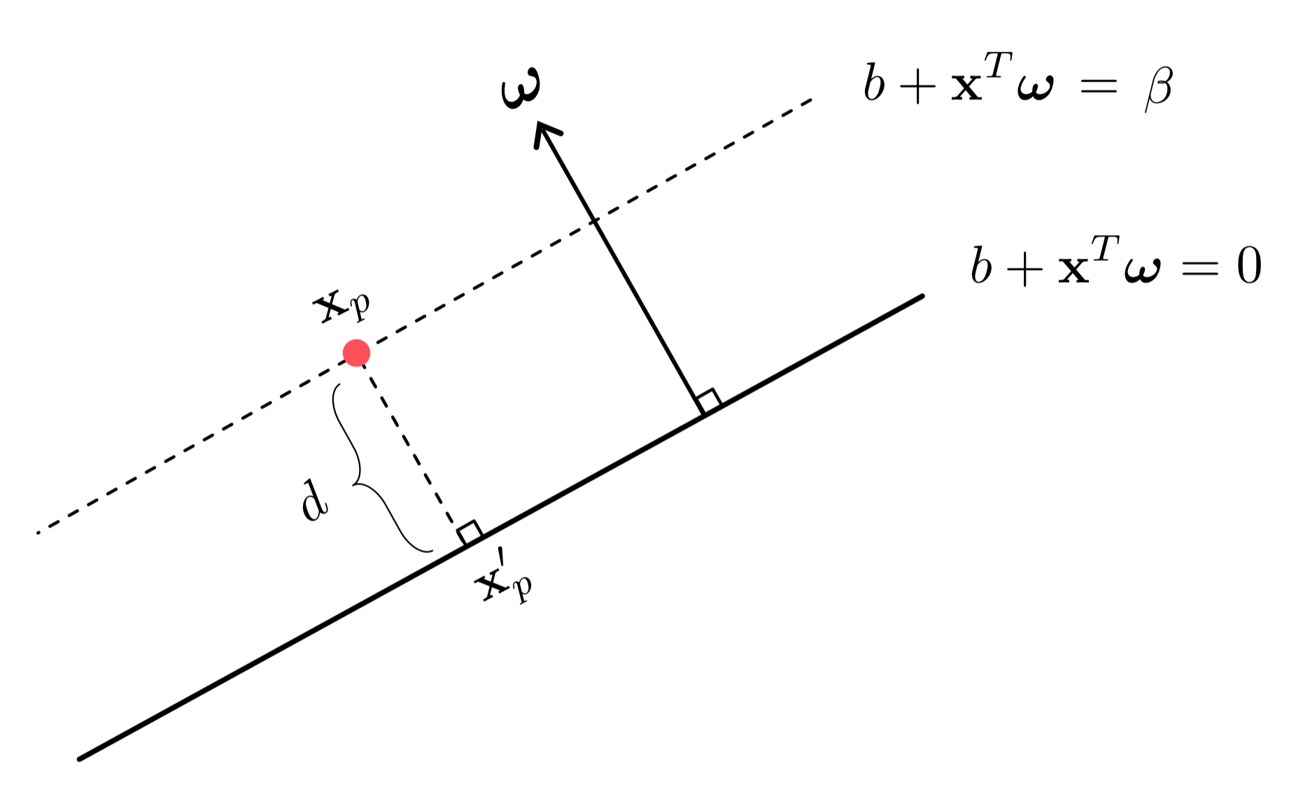
To see how this is possible, imagine we have a point $\mathbf{x}_p$ lying 'above' the linear decision boundary on a translate of the decision boundary where $b + \overset{\,}{\mathbf{x}}_{\,}^T\boldsymbol{\omega} = \beta > 0$, as illustrated in the Figure above. The same simple argument that follows can be made if $\mathbf{x}_p$ lies 'below' it as well. To compute the distance of $\mathbf{x}_p$ to the decision boundary imagine we know the location of its vertical projection onto the decision boundary which will call $\mathbf{x}_p^{\prime}$. To compute our desired error we want to compute the signed distance between $\mathbf{x}_p$ and its vertical projection, i.e., the length of the vector $\mathbf{x}_p^{\prime} - \mathbf{x}_p$ times the sign of $\beta$ which here is $+1$ since we assume the point lies above the decision boundary hence $\beta > 0$, i.e., $d = \left\Vert \mathbf{x}_p^{\prime} - \mathbf{x}_p \right\Vert_2 \text{sign}\left(\beta\right) = \left\Vert \mathbf{x}_p^{\prime} - \mathbf{x}_p \right\Vert_2$. Now, because this vector is also perpindicular to the decision boundary (and so is paralell to the normal vector $\boldsymbol{\omega}$) the inner-product rule gives
\begin{equation} \left(\mathbf{x}_p^{\prime} - \mathbf{x}_p\right)^T\boldsymbol{\omega} = \left\Vert \mathbf{x}_p^{\prime} - \mathbf{x}_p \right\Vert_2 \left\Vert \overset{\,}{\boldsymbol{\omega}} \right\Vert_2 = d\,\left\Vert \overset{\,}{\boldsymbol{\omega}} \right\Vert_2 \end{equation}
Now if we take the difference between our decision boundary and its translation evaluated at $\mathbf{x}_p^{\prime}$ and $\mathbf{x}_p$ respectively, we have simplifying
\begin{equation} \beta - 0 = \left(b + \left(\overset{\,}{\mathbf{x}}_{p}^{\prime}\right)^T \boldsymbol{\omega}\right)- \left(b + \overset{\,}{\mathbf{x}}_{p}^T \boldsymbol{\omega}\right) = \left(\mathbf{x}_p^{\prime} - \mathbf{x}_p\right)^T\boldsymbol{\omega} \end{equation}
Since both formulae are equal to $\left(\mathbf{x}_p^{\prime} - \mathbf{x}_p\right)^T\boldsymbol{\omega}$ we can set them equal to each other, which gives
\begin{equation} d\,\left\Vert \overset{\,}{\boldsymbol{\omega}} \right\Vert_2 = \beta \end{equation}
or in other words that the signed distance $d$ of $\mathbf{x}_p$ to the decision boundary is
\begin{equation} d = \frac{\beta}{\left\Vert \overset{\,}{\boldsymbol{\omega}} \right\Vert_2 } = \frac{b + \overset{\,}{\mathbf{x}}_{p}^T\boldsymbol{\omega} }{\left\Vert \overset{\,}{\boldsymbol{\omega}} \right\Vert_2 }. \end{equation}
Note that we need not worry dividing by zero here since if the feature-touching weights $\boldsymbol{\omega}$ were all zero, this would imply that the bias $b = 0$ as well and we have no decision boundary at all. Also notice, this analysis implies that if the feature-touching weights have unit length as $\left\Vert \boldsymbol{\omega}\right\Vert_2 = 1$ then the signed distance $d$ of a point $\mathbf{x}_p$ to the decision boundary is given simply by its evaluation $b + \mathbf{x}_p^T \boldsymbol{\omega}$. Finally note that if $\mathbf{x}_p$ were to lie below the decision boundary and $\beta < 0$ nothing about the final formulae derived above will change.
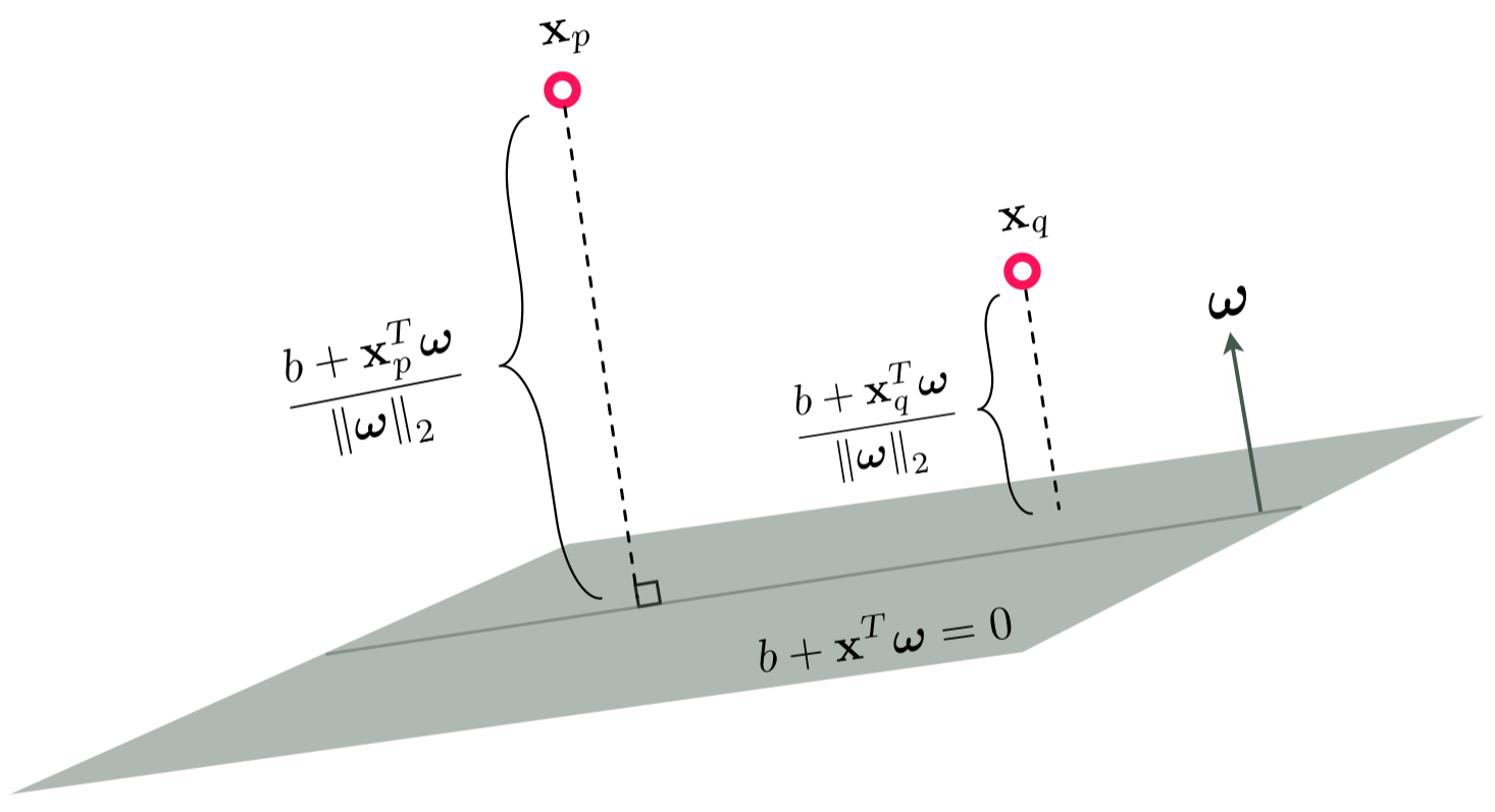
We mark this point-to-decision-boundary distance on points in the figure below, here the input dimension $N = 3$ and the decision boundary is a true hyperplane.
Remember, as detailed above, we can scale any linear decision boundary by a non-zero scalar $C$ and it still defines the same hyperplane. So if - in particular - we multiply by $C = \frac{1}{\left\Vert \overset{\,}{\boldsymbol{\omega}} \right\Vert_2}$ we have
\begin{equation} \frac{b + \overset{\,}{\mathbf{x}}_{\,}^T\boldsymbol{\omega} }{\left\Vert \overset{\,}{\boldsymbol{\omega}} \right\Vert_2 } = \frac{b}{\left\Vert \overset{\,}{\boldsymbol{\omega}} \right\Vert_2} + \overset{\,}{\mathbf{x}}_{\,}^T\frac{\boldsymbol{\omega}}{\left\Vert \overset{\,}{\boldsymbol{\omega}} \right\Vert_2} = 0 \end{equation}
we do not change the nature of our decision boundary and now our feature-touching weights have unit length as $\left\Vert \frac{\boldsymbol{\omega}}{\left\Vert \overset{\,}{\boldsymbol{\omega}} \right\Vert_2}\right \Vert_2 = 1$. In other words, regardless of how large our weights $\mathbf{w}$ were to begin with we can always normalize them in a consistent way by dividing off the magnitude of $\boldsymbol{\omega}$.
This normalization scheme is particularly useful in the context of the technical issue with the Softmax / Cross-entropy highlighted in the previous Subsection. because clearly a decision boundary that perfectly separates two classes of data can be feature-weight normalized to prevent its weights from growing too large (and diverging too infinity). Of coures we do not want to wait to perform this normaliation until after we run our local optimization, since this will not prevent the magnitude of the weights from potentially diverging, but during optimization.
With can achieve this by constraining the Softmax / Cross-Entropy cost so that feature-touching weights always have length one i.e., $\left\Vert \boldsymbol{\omega} \right\Vert_2 = 1$. Formally we can phrase this minimization (employing the Softmax cost) to as a constrained optimization problem as follows
\begin{equation} \begin{aligned} \underset{b, \,\boldsymbol{\omega}_{\,}}{\,\,\,\,\,\mbox{minimize}\,\,\,} & \,\,\,\, \frac{1}{P}\sum_{p=1}^P\text{log}\left(1 + e^{-y_p\left(b + \mathbf{x}_p^T \boldsymbol{\omega}^{\,}_{\,}\right)}\right) \\ \mbox{subject to}\,\,\, & \,\,\,\,\, \left \Vert \boldsymbol{\omega} \right \Vert_2^2 = 1 \end{aligned} \end{equation}
By solving this constrained version of the Softmax cost we can still learn a decision boundary that perfectly separates two classes of data, but we avoid divergence in the magnitude of the weights by keeping their magnitude feature-weight normalized.
This formulation can indeed be solved by simple extensions of the local optimization methods detailed in Chapters 2 -4 (see this Chapter's exercises for further details). However a more popular approach in the machine learning community is to 'relax' this constrinaed formulation and instead solve the highly related unconstrained problem. This relaxed form of the problem consists in minimizing a cost functionn that is a linear combination of our original Softmax cost the magnitude of the feature weights
\begin{equation} g\left(b,\boldsymbol{\omega}\right) = \frac{1}{P}\sum_{p=1}^P\text{log}\left(1 + e^{-y_p\left(b + \mathbf{x}_p^T \boldsymbol{\omega}^{\,}_{\,}\right)}\right) + \lambda\, \left \Vert \boldsymbol{\omega} \right \Vert_2^2 \end{equation}
which we can minimize using any of our familiar local optimization schemes. Note here the regularization parameter $\lambda \geq 0$. Here in adding the magnitude of the feature-touching weights to our Softmax cost we 'put pressure' on both terms, and aim to make both small. The parameter $\lambda$ is used to balance how strongly we pressure one term or the other. In minimizing the first term, our Softmax cost, we are still looking to learn an excellent linear decision boundary. In also minimizing the second term, the magnitude of the feature-touching weights $\lambda\, \left \Vert \boldsymbol{\omega} \right \Vert_2^2$ also called a regularizer - we incentivize the learning of small weights. This prevents the divergence of their magnitude since if their size does start to grow we our entire cost function 'suffers' because of it, and becomes large. Because of this the value of $\lambda$ is typically chosen to be small (and positive) in practice, although some fine-tuning can be useful.
Here we repeat the experiment of the previous Example, but add a regularizer with $\lambda = 10^(-3)$ to the Softmax cost. In the right panel below we show the contour plot of the regularized cost function, and we can see its global minimum no longer lies at infinity. However we still learn a perfect decision boundary as illustrated in the left panel by a tightly fitting $\text{tanh}\left(\cdot\right)$ function.
