code

share


In this Section we describe a fundamental framework for linear two-class classification called logistic regression, in particular employing the Cross Entropy cost function. Logistic regression follows naturally from the regression framework regression introduced in the previous Chapter, with the added consideration that the data output is now constrained to take on only two values.
Two class classification is a particular instance of regression or surface-fitting, wherein the output of a dataset of $P$ points $\left\{ \left(\mathbf{x}_{p},y_{p}\right)\right\} _{p=1}^{P}$ is no longer continuous but takes on two fixed numbers. The actual value of these numbers is in principle arbitrary, but particular value pairs are more helpful than others for derivation purposes (i.e., it is easier to determine a proper nonlinear function to regress on the data for particular output value pairs). Here we will use the values $y_{p}\in\left\{ 0,\,+1\right\}$ - that is every output takes on either the value $0$ or $+1$. Often in the context of classification the output values $y_p$ are called labels, and all points sharing the same label value are referred to as a class of data. Hence a dataset containing points with label values $y_{p}\in\left\{ 0,\,+1\right\}$ is said to be a dataset consisting of two classes.
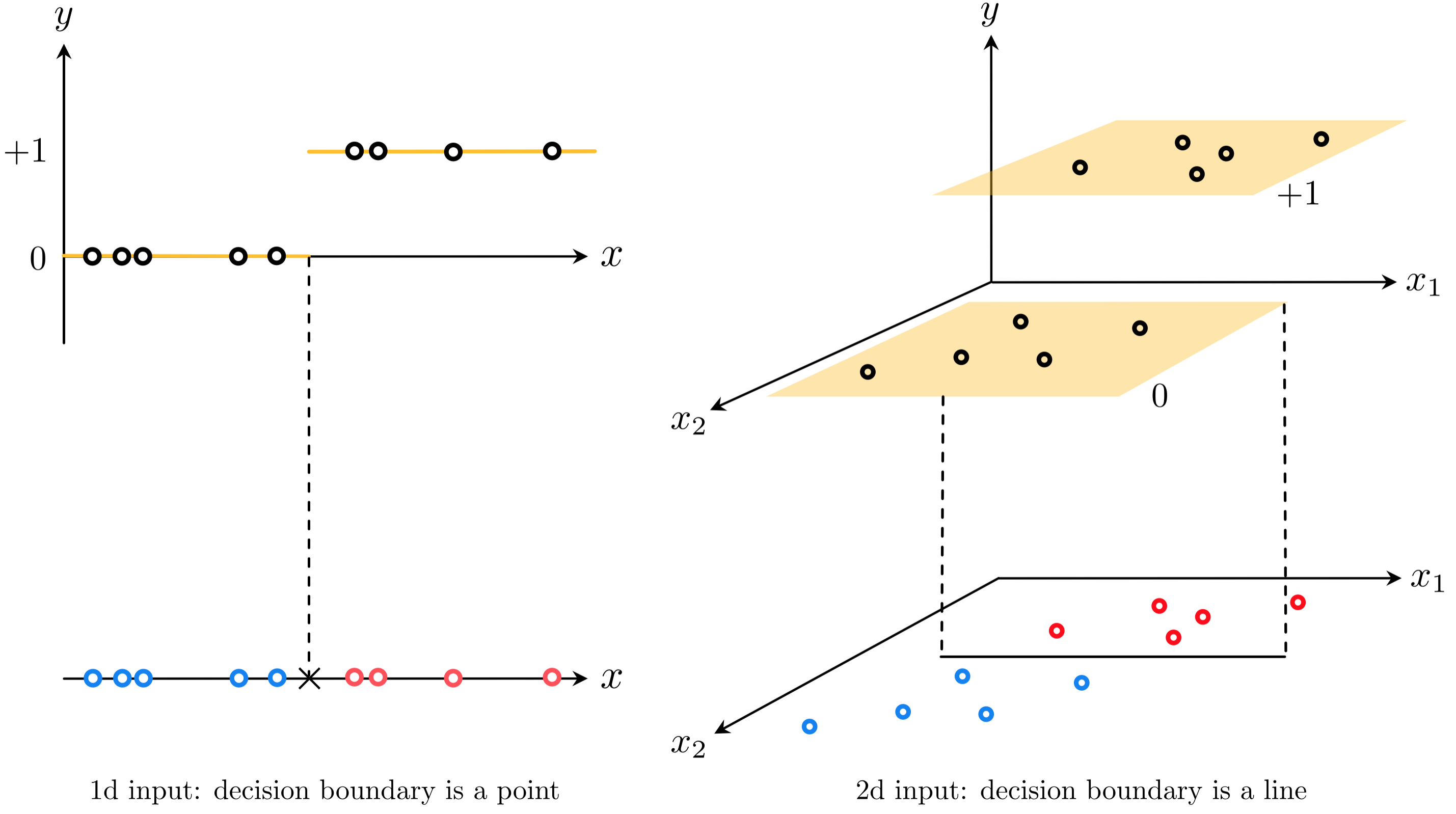
The simplest shape such a dataset can take is that of a set of linearly separated adjacent 'steps', as illustrated in the figure below. Here the 'bottom' step is the region of the space containing most of the points that have label value $y_p = 0$. The 'top step' likewise contains most of the points having label value $y_p = +1$. These steps are largely separated by a point when $N = 1$, a line when $N = 2$, and a hyperplane when $N$ is larger (the term 'hyperplane' is also used more generally to refer to a point or line as well).
As shown in the figure, because its output takes on a discrete set of values one can view a classification dataset 'from above', that is looking down from a point high up on the $y$ axis (or in other words, the data projected onto the plane $y = 0$). From this perspective we remove the vertical $y$ dimension of the data and visually represent the dataset using its input only, displaying the output values of each point by coloring its input one of two unique colors (we choose blue for points with label $y_p = 0$, and red for those having label $y_p = +1$).
This is the simplest sort of dataset with binary output we could aim to perform regression on, as in general the boundary between the two classes of data could certainly be nonlinear. We will deal with this more general potentiality later on - when discussing neural networks, trees, and kernel-based methods - but first let us deal with the current scenario. How can we perform regression on a dataset like the ones described in the figure above?
How can we fit a regression to data that is largely distributed on two adjacent steps separated by a hyperplane? Lets look at a simple instance of such a dataset when $N = 1$ to build our intuition about what must be done in general.
Intuitively it is obvious that simply fitting a line of the form $y = w_0 + w_1x_{\,}$ to such a dataset will result in an extremely subpar results - the line by itself is simply too inflexible to account for the nonlinearity present in the data. A dataset that is roughly distributed on two steps needs to be fit with a function that matches this general shape. In other words such data needs to be fit with a step function.
Since the boundary between the two classes is (assumed to be) linear and the labels take on values that are either $0$ or $1$, ideally we would like to fit a discontinuous step function with a linear boundary to such a dataset. What does such a function look like? When $N = 1$ a linear model defining this boundary is just a line $w_0 + x_{\,}w_1$ composed with the step function $\text{step}\left(\cdot\right)$ as
\begin{equation} \text{step}\left(w_0 + x_{\,}w_1 \right) \end{equation}
where the step function is defined as
\begin{equation} \text{step}(x) = \begin{cases} 1 \,\,\,\,\,\text{if} \,\, x \geq 0.5 \\ 0 \,\,\,\,\,\text{if} \,\, x < 0.5 \\ \end{cases}. \end{equation}
Note here that what happens with $\text{step}(0.5)$ is - for our purposes - arbitrary (i.e., it can be set to any fixed value or left undefined as we have done). The linear boundary between the two steps is defined by all points $x$ where $w_0 + xw_1 = 0.5$.
More generally with general $N$ dimensional input we can write the liinear model defining the boundary employing our compact vector notation first introduced in Section 5.2
\begin{equation} \mathbf{w}= \begin{bmatrix} w_{0}\\ w_{1}\\ w_{2}\\ \vdots\\ w_{N} \end{bmatrix} \,\,\,\,\,\text{and}\,\,\,\,\,\, \mathring{\mathbf{x}}_{\,}= \begin{bmatrix} 1\\ x_{1}\\ x_{2}\\ \vdots\\ x_{N} \end{bmatrix}. \end{equation}
as
\begin{equation} \mathring{\mathbf{x}}_{\,}^T\mathbf{w}^{\,} = w_{0}+ x_{1}w_{1} + x_{2}w_{2} + \cdots + x_{N}w_{N} . \end{equation}
A corresponding step function is then simply the $\text{step}\left(\cdot\right)$ of this linear combination
\begin{equation} \text{step}\left(\mathring{\mathbf{x}}_{\,}^T\mathbf{w}^{\,}\right) \end{equation}
and the linear boundary between the steps is defined by all points $\mathring{\mathbf{x}}_{\,}$ where $\mathring{\mathbf{x}}_{\,}^T\mathbf{w}^{\,} = 0.5$.
How do we tune the parameters of the line? We could try to take the lazy way out and first fit the line to the classification dataset via linear regression, then compose the line with the step function to get a step function fit. However this does not work well in general - as we will see even in the simple instance below. Instead we need to tune the parameters $w_0$ and $w_1$ after composing the linear model with the step function, or in other words we need to tune the parameters of $\text{step}\left(\mathring{\mathbf{x}}_{\,}^T\mathbf{w}^{\,}\right)$.
In the Python cell below we load in a simple two-class dataset (top panel), fit a line to this dataset via linear regression, and then compose the fitted line with the step function to produce a step function fit. Both the linear fit (in green) as well as its composition with the step function (in dashed red) are shown along with the data in the bottom panel. Of course the line itself provides a terrible representation of the nonlinear dataset. But its evaluation through the step is also quite poor for such a simple dataset, failing to properly identify two points on the top step. In the parlance of classification these types of points are referred to as misclassified points.

How do we tune these parameters properly? As with linear regression, here we can try to setup a proper Least Squares function that - when minimized - recovers our ideal weights. We can do this by simply reflecting on the sort of ideal relationship we want to find between the input and output of our dataset.
Take a single point $\left(\mathbf{x}_p,\,y_p \right)$. Notice in the example above - and this is true more generally speaking - that ideally for a good fit we would like our weights to be such if this point has a label $+1$ it lies in the positive region of the space where $\mathring{\mathbf{x}}_{\,}^T\mathbf{w}^{\,} > 0.5$ so that $\text{step}\left(\mathring{\mathbf{x}}_{\,}^T\mathbf{w}^{\,}\right) = +1$ matches its label value. Likewise if this point has label $0$ we would like it to lie in the negative region where $\mathring{\mathbf{x}}_{\,}^T\mathbf{w}^{\,}< 0.5$ so that $\text{step}\left(\mathring{\mathbf{x}}_{\,}^T\mathbf{w}^{\,}\right) = 0$ matches its label value. So in short what we would ideally like for this point is that its evaluation matches its label value, i.e., that
\begin{equation} \text{step}\left(\mathring{\mathbf{x}}_{p}^T\mathbf{w}^{\,}\right)= y_p^{\,}. \end{equation}
And of course we would like this to hold for every point. To find weights that satisfy this set of $P$ equalities as best as possible we could - as we did previously with linear regression - square the difference between both sides of each and average them, giving the Least Squares function
\begin{equation} g(\mathbf{w}) = \frac{1}{P}\sum_{p=1}^P \left(\text{step}\left(\mathring{\mathbf{x}}_{\,}^T\mathbf{w}^{\,}\right) - y_p \right)^2 \end{equation}
which we can try to minimize in order to recover weights that satisfy our desired equalities. If we can find a set of weights such that $g(\mathbf{w}) = 0$ then all $P$ equalities above hold true, otherwise some of them do not.
Unfortunately because this Least Squares cost takes on only integer values it is impossible to minimize with our gradient-based techniques, as at every point the function is completely flat, i.e., it has exactly zero gradient. Because of this neither gradient descent nor Newton's method can take a single step 'downhill' regardless of where they are initialized. This problem is inherited from our use of the step function, itself a discontinuous step.
In the next Python cell we plot the Least Squares in equation (4) (left panel) for the dataset displayed in Example 1, over a wide range of values for $w_0$ and $w_1$. This Least Squares surface consists of discrete steps at many different levels, each one completely flat. Because of this no local method can be used to minimize the counting cost.
In the middle and right panels we plot the surfaces of two related cost functions on the same dataset. We introduce the cost function shown in the middle panel in the next subection, and the cost in the right panel in the one that follows. We can indeed minimize either of these using a local method to recover ideal weights.

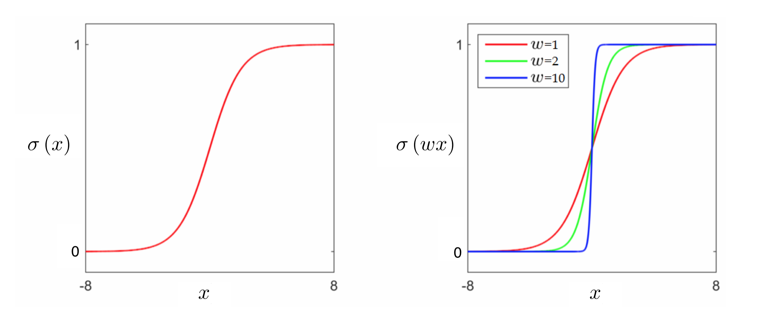
As mentioned above, we cannot directly minimize the Least Squares above due to our use of the step function. In other words, we cannot directly fit a discontinuous step function to our data. In order to go further we need to replace the step function, ideally with a continuous function that matches it very closely everywhere. Thankfully such a function is readily available: the sigmoid function, $\sigma(\cdot)$
\begin{equation} \sigma\left(x\right) = \frac{1}{1 + e^{-x}}. \end{equation}
This kind of function is alternatively called a logistic function - and when we fit such a function to a classification dataset we are therefore performing regression with a logistic or logistic regression.
In the figure below we plot the sigmoid function (left panel), as well as several internally weighted versions of it (right panel). As we can see in the figure, for the correct setting of internal weights the hyperbolic tangent function can be made to look arbitrarily similar to the step function.
Swapping out the step function with sigmoid in equation (5) we aim to satisfy as many of the $P$ equations
\begin{equation} \sigma\left(\mathring{\mathbf{x}}_{\,}^T\mathbf{w}^{\,}\right) = y_p \,\,\,\,\,\,\,\,\,\,\,\,\,\,\,\,\,\, p=1,..,P \end{equation}
as possible. To learn parameters that force these approximations to hold we can do precisely what we did in the case of linear regression: try to minimize the e.g., the squared error between both sides constructing the Least Squares point-wise cost
\begin{equation} g_p\left(\mathbf{w}\right) = \left(\sigma\left(\mathring{\mathbf{x}}_{p}^T\mathbf{w}^{\,}\right) - y_p \right)^2 \,\,\,\,\,\,\,\,\,\,\,\,\,\,\,\,\,\, p=1,..,P. \end{equation}
Taking the average of these squared errors gives a Least Squares cost for logistic regression
\begin{equation} g\left(\mathbf{w}\right) = \frac{1}{P}\sum_{p=1}^P \left(\sigma\left(\mathring{\mathbf{x}}_{\,}^T\mathbf{w}^{\,} \right) - y_p \right)^2 \end{equation}
This function - an example of which is plotted in the previous example - is generally non-convex and contains large flat regions. Because of this - as we saw in Chapters 3 and 4 - this sort of function is not easily minimized using stanard gradient descent or Newtons method algorithms. Specialized algorithms - like the normalized gradient descent scheme presented in Section 3.9 - can be employed successfully as we show in the example below. However it is more commonplace to simply employ a different and convex cost function based on the set of desired approximations in equation (4). We do this following the example.
In this example we show how normalized gradient descent can be used to minimize the logistic Least Squares cost, translated into Python in the next cell.
# define sigmoid function
def sigmoid(t):
    return 1/(1 + np.exp(-t))

# sigmoid non-convex logistic least squares cost function
def sigmoid_least_squares(w):
    cost = 0
    for p in range(y.size):
        x_p = x[:,p]
        y_p = y[:,p]
        cost += (sigmoid(w[0] + w[1]*x_p) - y_p)**2
    return cost/y.size
First, we load in a simulated one-dimensional dataset (left panel) and plot its corresponding tanh Least Squares cost (right panel).

We now run normalized gradient descent for $900$ iterations, initialized at $w_0=-w_1=20$, with steplength parameter fixed at $\alpha=1$.
The cell below plots the Least Squares logistic regression fit to the data (left panel) along with the gradient descent path towards the minimum on the contour plot of the cost function (right panel). The normalized gradient descent steps are colored green to red as the run progresses.

There is more than one way to form a cost function whose minimum forces as many of the $P$ equalities in equation (4) to hold as possible. The squared error / point-wise cost $g_p\left(\mathbf{w}\right) = \left(\sigma\left(\mathring{\mathbf{x}}_{p}^T\mathbf{w}^{\,} \right) - y_p\right)^2$ penalty works universally, regardless of the values taken by the output by $y_p$. However because we know that the output we deal with now is limited to the discrete values $y_p \in \left\{0,1\right\}$ it is reasonable to ask if we cannot create a more appropriate cost that is customized to deal with just such output.
Such a point-wise cost does exist for these restricted output values. One such cost - which we call the Log Error - is as follows
\begin{equation} g_p\left(\mathbf{w}\right)= \begin{cases} -\text{log}\left(\sigma\left( \mathring{\mathbf{x}}_{p}^T\mathbf{w}^{\,} \right) \right) \,\,\,\,\,\,\,\,\,\, \,\,\,\, \text{if} \,\, y_p = 1 \\ -\text{log}\left(1 - \sigma\left( \mathring{\mathbf{x}}_{p}^T\mathbf{w}^{\,} \right) \right) \,\,\,\,\,\text{if} \,\, y_p = 0. \\ \end{cases} \end{equation}
First notice that regardless of the weight values this point-wise cost is always nonnegative and takes on a minimum value at $0$. Second notice how this penalizes violations of our desired equalities in equation (4) (and much more harshly than a Least Squares cost too). A plot showing both the Least Squares and Log Error point-wise costs are shown below.

Suppose we have our optimally tuned our weights and that $y_p = 1$. Then with our ideal weights we should satisfy our desired equality and have $\sigma\left(\mathring{\mathbf{x}}_{\,}^T\mathbf{w}^{\,}\right) \approx y_p = 1$, and if this indeed the case then $-\text{log}\left(\sigma\left(\mathring{\mathbf{x}}_{\,}^T\mathbf{w}^{\,}\right) \right) \approx -\text{log}\left(1\right) = 0$ which is a neglibable penalty. However if $\sigma\left(\mathring{\mathbf{x}}_{\,}^T\mathbf{w}^{\,}\right) < 1$ the value $-\text{log}\left(\sigma\left(\mathring{\mathbf{x}}_{\,}^T\mathbf{w}^{\,}\right) \right)$ becomes large and positive very quickly harshly penalizing violations of our desired equality. As $\sigma\left(\mathring{\mathbf{x}}_{\,}^T\mathbf{w}^{\,}\right) $ approaches $0$ - the worst possible value it could take on if indeed $y_p = 1$ - then cost value goes to positive infinity. So indeed, this point-wise cost function penalizes violations when $y_p = 1$ very strictly and is minimal (equals $0$) in value when the desired equality holds. Precisely the same thing can be said when $y_p = 0$, that this point-wise cost takes on a minimal value when $\sigma\left(\mathring{\mathbf{x}}_{\,}^T\mathbf{w}^{\,}\right) \approx 0$ and is very large otherwise going to positive infinity as $\sigma\left(\mathring{\mathbf{x}}_{\,}^T\mathbf{w}^{\,}\right) $ approaches the worst possible value of $1$.
So - in short - point-wise cost severely punishes violations of our desired equalitiesa and takes on a minimum value of $0$ when our weights $\mathbf{w}$ are properly tuned i.e.,
\begin{equation} g_p\left(\mathbf{w}\right)\approx 0. \end{equation}
We can then form the so-called Cross Entropy cost function by taking the average of the Log Error costs over all $P$ points as
\begin{equation} g\left(\mathbf{w}\right) = \frac{1}{P}\sum_{p=1}^P g_p\left(\mathbf{w}\right). \end{equation}
Finally notice that we can write the Log Error equivalently - combining the two cases - in a single line as
\begin{equation} g_p\left(\mathbf{w}\right)= -y_p\,\text{log}\left(\sigma\left(\mathring{\mathbf{x}}_{p}^T\mathbf{w}^{\,}\right) \right) -\left(1-y_p\right)\text{log}\left(1 -\sigma\left(\mathring{\mathbf{x}}_{p}^T\mathbf{w}^{\,}\right) \right). \end{equation}
We can form the same cost function as above by taking the average of this form of the Log Error giving
\begin{equation} g\left(\mathbf{w}\right) = \frac{1}{P}\sum_{p=1}^P g_p\left(\mathbf{w}\right) = - \frac{1}{P}\sum_{p=1}^P y_p\,\text{log}\left(\sigma\left(\mathring{\mathbf{x}}_{p}^T\mathbf{w}^{\,}\right) \right) +\left(1-y_p\right)\text{log}\left(1 - \sigma\left(\mathring{\mathbf{x}}_{p}^T\mathbf{w}^{\,}\right) \right) \end{equation}
which is the more common way of expressing the Cross Entropy cost.
In any case, to recover the ideal weights that make the formulae in equation (4) hold as tightly as possible we want to minimize this cost over $\mathbf{w}$. In other words, to optimally tune the parameters $\mathbf{w}$ we want to minimize the Cross Entropy cost as
\begin{equation} \underset{\mathbf{w}}{\mbox{minimize}}\,\, -\frac{1}{P}\sum_{p=1}^P y_p\,\text{log}\left(\sigma\left(\mathring{\mathbf{x}}_{p}^{T}\mathbf{w}^{\,}\right)\right) + \left(1 - y_p\right)\text{log}\left(1 - \sigma\left(\mathring{\mathbf{x}}_{p}^{T}\mathbf{w}^{\,}\right)\right) \end{equation}
since the smaller this cost function becomes the better we have tuned our parameters $\mathbf{w}$.
The Cross Entropy cost is always convex regardless of the dataset used - we will see this empirically in the examples below and a mathematical proof is provided in the appendix of this Section that verifies this claim more generally. We displayed a particular instance of the cost surface in the right panel of Example 2 for the dataset first shown in Example 1. Looking back at this surface plot we can see that it is indeed convex.
Since the Cross Entropy cost function is convex a variety of local optimization schemes can be more easily used to properly minimize it. For this reason the Cross Entropy cost is used more often in practice for logistic regression than is the logistic Least Squares cost.
Python¶We can implement the Cross Entropy costs very similarly to the way we did the Least Sqwuares cost for linear regression, as detailed in Section 5.2, breaking down our implementation into the linear model and the error itself. Our linear model takes in both an appended input point $\mathring{\mathbf{x}}_p$ and a set of weights $\mathbf{w}$
\begin{equation} \text{model}\left(\mathbf{x}_p,\mathbf{w}\right) = \mathring{\mathbf{x}}_{p}^{T}\mathbf{w}^{\,}. \end{equation}
With this notation for our model, the corresponding Cross Entropy cost in equation (16) can be written
\begin{equation*} g(\mathbf{w}) = -\frac{1}{P}\sum_{p=1}^P y_p\text{log}\left(\sigma\left(\text{model}\left(\mathbf{x}_p,\mathbf{w}\right)\right)\right) + \left(1 - y_p\right)\text{log}\left(1 - \sigma\left(\text{model}\left(\mathbf{x}_p,\mathbf{w}\right)\right)\right) \end{equation*}
We can then implement the cost in chunks - first the model function below precisely as we did with linear regression.
# compute linear combination of input point
def model(x,w):
    a = w[0] + np.dot(x.T,w[1:])
    return a.T
We can then implement the Cross Entropy cost function by e.g., implementing the Log Loss error and employing efficient and compact numpy operations as
# define sigmoid function
def sigmoid(t):
    return 1/(1 + np.exp(-t))

# the convex cross-entropy cost function
def cross_entropy(w):
    # compute sigmoid of model
    a = sigmoid(model(x,w))

    # compute cost of label 0 points
    ind = np.argwhere(y == 0)[:,1]
    cost = -np.sum(np.log(1 - a[:,ind]))

    # add cost on label 1 points
    ind = np.argwhere(y==1)[:,1]
    cost -= np.sum(np.log(a[:,ind]))

    # compute cross-entropy
    return cost/y.size
To minimize this cost we can use virtually any local optimization method detailed in Chapters 2 - 4. For first and second order methods (e.g., standard gradient descent and Newton's method schemes) an Automatic Differentiator can be used - e.g., employing autograd as detailed in Section 3.5 - to properly compute its gradient and Hessian.
Alternatively one can indeed compute the gradient and Hessian of the Cross Entropy cost in closed form, and implement them directly. Using the simple derivative rules outlined in the Appendix of this text the gradient can be computed as
\begin{equation} \nabla g\left(\mathbf{w}\right) = - \frac{1}{P}\sum_{p = 1}^P\left(y_p - \sigma\left(\mathring{\mathbf{x}}_{p}^{T}\mathbf{w}^{\,}\right)\right) \mathring{\mathbf{x}}_{p} \end{equation}
In addition to employ Newton's method 'by hand' one can hand compute the Hessian of the Cross Entropy function as
\begin{equation} \nabla^2 g\left(\mathbf{w}\right) = \frac{1}{P}\sum_{p = 1}^P \sigma\left(\mathring{\mathbf{x}}_{p}^{T}\mathbf{w}^{\,}\right)\left(1 - \sigma\left(\mathring{\mathbf{x}}_{p}^{T}\mathbf{w}^{\,}\right)\right) \mathring{\mathbf{x}}_p^{\,}\mathring{\mathbf{x}}_p^T. \end{equation}
In this example we repeat the experiments of Example 2 using the Cross Entropy cost and gradient descent.
With our cost function defined in Python we can now run our demonstration. We initialize at the point $w_0 = 3$ and $w_1 =3$, set $\alpha = 1$, and run for 25 steps.
Each step of the run is now animated - along with its corresponding fit to the data. In the left panel both the data and the fit at each step (colored green to red as the run continues) are shown, while in the right panel the contour of the cost function is shown with each step marked (again colored green to red as the run continues). Moving the slider from left to right animates the run from start to finish. Note how we still have some zig-zagging behavior here, but since we can safely use unnormalized gradient descent, its oscillations rapidly decrease in magnitude since the length of each step is directly controlled by the magnitude of the gradient.
Below we show the result of running gradient descent with the same initial point and fixed steplength parameter for $2000$ iterations, which results in a better fit.

To show that the Cross Entropy cost function is convex we can use the second order definition of convexity, by which we must show that the eigenvalues of this cost function's Hessian matrix are all always nonnegative. Studying the Hessian of the cros-entropy - which was defined algebraically in Example 4 above - we have
\begin{equation} \nabla^2 g\left(\mathbf{w}\right) = \frac{1}{P}\sum_{p = 1}^P \sigma\left(\mathring{\mathbf{x}}_{p}^{T}\mathbf{w}^{\,}\right)\left(1 - \sigma\left(\mathring{\mathbf{x}}_{p}^{T}\mathbf{w}^{\,}\right)\right) \mathring{\mathbf{x}}_p^{\,}\mathring{\mathbf{x}}_p^T. \end{equation}
We know that the smallest eigenvalue of any square symmetric matrix is given as the minimum of the Rayleigh quotient (as detailed Section 3.2), i.e., the smallest value taken by
\begin{equation} \mathbf{z}^T \nabla^2 g\left(\mathbf{w}\right) \mathbf{z}^{\,} \end{equation}
for any unit-length vector $\mathbf{z}$ and any possible weight vector $\mathbf{w}$. Substituting in the particular form of the Hessian here, denoting $\sigma_p = \sigma\left(\mathring{\mathbf{x}}_{p}^{T}\mathbf{w}^{\,}\right)\left(1 - \sigma\left(\mathring{\mathbf{x}}_{p}^{T}\mathbf{w}^{\,}\right)\right) $ for each $p$ for short, we have
\begin{equation} \mathbf{z}^T \nabla^2 g\left(\mathbf{w}\right) \mathbf{z}^{\,}= \mathbf{z}^T \left(\frac{1}{P} \sum_{p=1}^{P}\sigma_p \mathbf{x}_p^{\,}\mathbf{x}_p^T\right) \mathbf{z}^{\,} = \frac{1}{P}\sum_{p=1}^{P}\sigma_p \left(\mathbf{z}^T\mathbf{x}_{p}^{\,}\right)\left( \mathbf{x}_{p}^T \mathbf{z}^{\,} \right) = \frac{1}{P}\sum_{p=1}^{P} \sigma_p \left(\mathbf{z}^T\mathbf{x}_{p}^{\,}\right)^2 \end{equation}
Since it is always the case that $\left(\mathbf{z}^T\mathbf{x}_{p}^{\,}\right)^2 \geq 0$ and $\sigma_p \geq 0$, it follows that the smallest value the above can take is $0$, meaning that this is the smallest possible eigenvalue of the softmax cost's Hessian. Since this is the case, the softmax cost must be convex.
Building on the analysis above showing that the cross-entropy cost is convex, we can likewise compute its largest possible eigenvalue by noting that the largest value $\sigma_p$ (defined previously) can take is $\frac{1}{4}$
\begin{equation} \sigma_k \leq \frac{1}{4} \end{equation}
Thus the largest value the Rayleigh quotient can take is bounded above for any $\mathbf{z}$ as
\begin{equation} \mathbf{z}^T \nabla^2 g\left(\mathbf{w}\right) \mathbf{z}^{\,} \leq \frac{1}{4P}\mathbf{z}^T \left(\sum_{p=1}^{P}\mathring{\mathbf{x}}_p^{\,}\mathring{\mathbf{x}}_p^T \right) \mathbf{z}^{\,} \end{equation}
Since the maximum value $\mathbf{z}^T \left(\sum_{p=1}^{P}\mathring{\mathbf{x}}_p^{\,}\mathring{\mathbf{x}}_p^T \right) \mathbf{z}^{\,}$ can take is the maximum eigenvalue of the matrix $\sum_{p=1}^{P}\mathring{\mathbf{x}}_p^{\,}\mathring{\mathbf{x}}_p^T $, thus a Lipschitz constant for the Cross Entropy cost is given as
\begin{equation} L = \frac{1}{4P}\left\Vert \sum_{p=1}^{P}\mathring{\mathbf{x}}_p^{\,}\mathring{\mathbf{x}}_p^T \right\Vert_2^2 \end{equation}