In this Section we describe simple metrics for judging the quality of a trained regression model, as well as how to make predictions using one.

Making predictions using a trained model

If we denote the optimal set of weights found by minimizing a regression cost function by $\mathbf{w}^{\star}$ then note we can write our fully tuned linear model as

\begin{equation} \text{model}\left(\mathbf{x},\mathbf{w}^{\star}\right) = \mathring{\mathbf{x}}_{\,}^T\mathbf{w}^{\star} = w_0^{\star} + x_{1}^{\,}w_1^{\star} + x_{2}^{\,}w_2^{\star} + \cdots + x_{N}^{\,}w_N^{\star}. \end{equation}

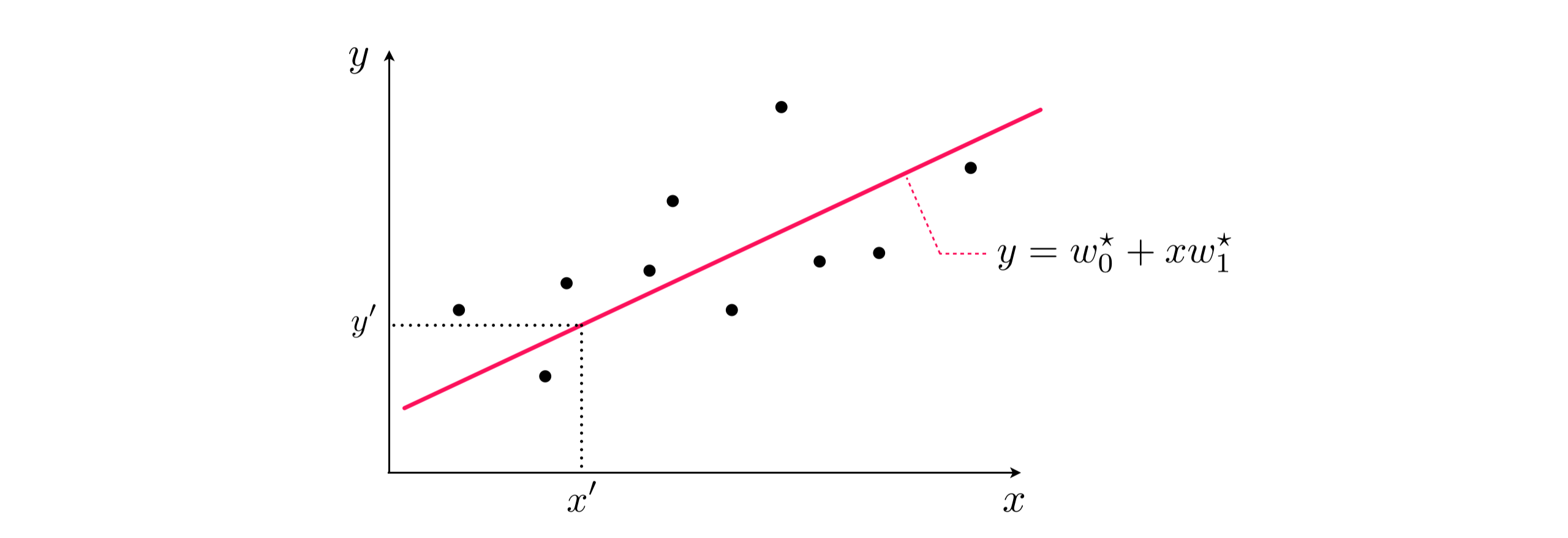
Regardless of how we determine optimal parameters $\mathbf{w}^{\star}$, by minimizing a regression cost like the Least Squares or Least Absolute Deviations, we make predictions employing our linear model in the same way. That is, given an input (whether one from our training dataset or a new input) $\mathbf{x}_{\,}$ we predict its output $y_{\,}$ by passing it along with our trained weigths into our model as

\begin{equation} \text{model}\left(\mathbf{x}_{\,},\mathbf{w}^{\star}\right) = y_{\,} \end{equation}

This is illustrated pictorially on a prototypical linear regression dataset for the case when $N=1$ in the Figure below.

Figure 4: Once a line/hyperplane has been fit to a dataset via minimizing an appropriate cost function it may be used to predict the output value of any input. Here a line has been fit to a two dimensional dataset in this manner, giving optimal parameters $w_0^{\star}$ and $w_1^{\star}$, and the output value of a new point $x^{\prime}$ is made using the learned linear model as $w_0^{\star}+x^{\prime}w_1^{\star} = y^{\prime}$.

Judging the quality of a trained model

Once we have successfully minimized the a cost function for linear regression it is an easy matter to determine the quality of our regression model: we simply evaluate a cost function using our optimal weights.

We can then evalaute the quality of this trained model using a Least Squares cost - which is especially natural to use when we employ this cost in training. To do this we plug in our trained model and dataset into the Least Squares cost - giving the Mean Squared Error (or MSE for short) of our trained model

\begin{equation} \text{MSE}=\frac{1}{P}\sum_{p=1}^{P}\left(\text{model}\left(\mathbf{x}_p,\mathbf{w}^{\star}\right) -y_{p}^{\,}\right)^{2}. \end{equation}

The name for this quality measurement describes precisely what the Least Squares cost computes - the average (or mean) squared error.

In the same way we can employ the Least Absolute Deviations cost to determine the quality of our trained model. Plugging in our trained model and dataset into this cost computes the Mean Absolute Deviations (or MAD for short) which is precisely what this cost function computes

\begin{equation} \text{MAD}=\frac{1}{P}\sum_{p=1}^{P}\left\vert\text{model}\left(\mathbf{x}_p,\mathbf{w}^{\star}\right) -y_{p}^{\,}\right\vert. \end{equation}

These two measurements differ in precisely the ways we have seen their respective cost functions differ - e.g., the MSE measure is far more sensitive to outliers. Which measure one employs in practice can therefore depend on personal and/or occupational preference, or the nature of a problem at hand.

Of course in general the lower one can make a quality measures, by proper tuning of model weights, the better the quality of the corresponding trained model (and vice versa). However the threshold for what one considers 'good' or 'great' performance can depend on personal preference, an occupational or institutionally set benchmark, or some other problem-dependent concern.

Implementing a fully trained model in Python

Given a Pythonic implementation of any local optimization scheme (detailed in Chapters 2 - 5) and a regression cost (as detailed in the first two Sections of this Chapter), we can easily implement a fully trained model in Python for predictive use. To do this suppose that weight_history and cost_history are two lists containing a history of weight steps and corresponding cost function evaluations returned by a local optimization scheme, then we first must determine which step provided the lowest cost function value. We do this below, calling the step at which a minimum cost value was achieved w_best.

# find the index of the step at which the smallest cost function value was attained
# and pluck out the corresponding set of weights from a local optimization run
ind = np.argmin(cost_history)
w_best = weight_history[ind]

Now given we have implemented a Pythonic version of our model, as detailed in previous Sections, our fully trained model is simply this function evaluated using w_best: that is to evaluate a new point x we evaluate model(x,w_best). For ease of use one can define a simple Python wrapper on this trained model functionality as shown below, which we call predict (short for fully trained predictor or model). This allows predictions on a new x to be made by simply calling predict(x).

# wrapper on fully trained model functionality
def predict(x):
    return model(x,w_best)