code

share


Since the first order Taylor series approximation to a function leads to the local optimization framework of gradient descent, it seems intuitive that higher order Taylor series approximations might similarly yield descent-based algorithms as well. In this Section we introduce a local optimization scheme based on the second order Taylor series approximation - called Newton's method. Because it is based on the second order approximation Newton's method has natural strengths and weaknesses when compared to gradient descent. In summary we will see that the cumulative effect of these trade-offs is - in general - that Newton's method is especially useful for minimizing convex functions of a moderate number of inputs.
The second order Taylor series approximation of a single input functions $g(w)$ at a particular point $v$ is a quadratic function of the form
\begin{equation} h(w) = g(v) + \left(\frac{\mathrm{d}}{\mathrm{d}w}g(v)\right)(w - v) + \frac{1}{2}\left(\frac{\mathrm{d}^2}{\mathrm{d}w^2}g(v)\right)(w - v)^2 \end{equation}
which is - typically speaking - a much better approximation of the underlying function near $v$ than is the first order Taylor series approximation on which gradient descent is built.
Below we produce an animation visualizing a single-input function $g(w) = \text{sin}(2w)$, along with its first and second order Taylor series approximation. As the animation plays the point $v$ (shown as a red dot) on which the approximations is based moves left to right, producing new approximations (the point on the graph of $g$ at which the approximations are tangent is marked with a small red 'x'). One can see that at each point the second order approximation (in blue) - since it contains both first and second derivative information at the point - is a much better local approximator than the first order analog (in green).
Note how the second order approximation matches the local convexity/concavity of the function $g$, i.e., where $g$ is convex/concave so too is the quadratic approximation.
# load video into notebook
from IPython.display import HTML
HTML("""
<video width="1000" height="400" controls loop>
  <source src="videos/animation_5.mp4" type="video/mp4">
  </video>
""")
This natural quadratic approximation generalizes for functions $g(\mathbf{w})$ taking in $N$ inputs, where at a point $\mathbf{v}$ the analogous second order Taylor series approximation looks like
\begin{equation} h(\mathbf{w}) = g(\mathbf{v}) + \nabla g(\mathbf{v})^T(\mathbf{w} - \mathbf{v}) + \frac{1}{2}(\mathbf{w} - \mathbf{v})^T \nabla^2 g\left(\mathbf{v}\right) (\mathbf{w} - \mathbf{v}) \end{equation}
where $\nabla g(\mathbf{v})$ is the gradient vector of first order partial derivatives, and $\nabla^2 g(\mathbf{v})$ is the $N\times N$ Hessian matrix containing second order partial derivatives of $g$ at $\mathbf{v}$. Like the analogous single-input version, this quadratic is a much better local approximator of $g$ near the point $\mathbf{v}$, matching its convexity/concavity there (i.e., if $g$ is convex/concave at $\mathbf{v}$ so too is the second order approximation).
Below we show an example comparing first and second order approximations (in green and blue respectively) using the sinusoid $g(w_1,w_2) = \text{sin}\left(w_1\right)$ at the point $\mathbf{v} = \begin{bmatrix} -1.5 \\ 1 \end{bmatrix}$. Clearly the second order approximation provides a better local representation of the function here.

In analogy to gradient descent, what would it mean to move in the 'descent direction' defined by the second order approximation at $\mathbf{v}$? Well unlike a hyperplane, a quadratic does not itself have such a descent direction. However it does have stationary points which are global minima when the quadratic is convex. Like the descent direction of a hyperplane, we can actually compute the stationary point(s) fairly easily using the first order condition for optimality (described in Section 3.2).
For the single input case of the second order Taylor series approximation centered at a point $v$ we can solve for the stationary point of the quadratic approximation by setting the first derivative of $h(w)$ to zero and solving. Doing this we compute the point $w^{\star}$
\begin{equation} w^{\star} = v - \frac{\frac{\mathrm{d}}{\mathrm{d}w}g(v)}{\frac{\mathrm{d}^2}{\mathrm{d}w^2}g(v)} \end{equation}
Note that this update says that to get to the point $w^{\star}$ we move from $v$ in the direction given by $- \frac{\frac{\mathrm{d}}{\mathrm{d}w}g(v)}{\frac{\mathrm{d}^2}{\mathrm{d}w^2}g(v)}$.
The same kind of calculation can be made in the multi-input case. Setting the gradient of the quadratic approximation to zero and solving gives the stationary point $\mathbf{w}^{\star}$ where
\begin{equation} \mathbf{w}^{\star} = \mathbf{v} - \left(\nabla^2 g(\mathbf{v})\right)^{-1}\nabla g(\mathbf{v}) \end{equation}
This is the direct analog of the single-input solution, and indeed reduces to it when $N=1$. It likewise says that in order to get to the new point $\mathbf{w}^{\star}$ we move from $\mathbf{v}$ in the direction $- \left(\nabla^2 g(\mathbf{v})\right)^{-1}\nabla g(\mathbf{v})$.
So in this notation, what might happen if we have a general function $g(\mathbf{w})$ and at the point $\mathbf{v}$ we form the second order Taylor series approximation there, calculate a stationary point $\mathbf{w}^{\star}$ of this quadratic, and move to it from $\mathbf{v}$? When might this lead us to a lower point on $g$? In other words, when might $- \left(\nabla^2 g(\mathbf{v})\right)^{-1}\nabla g(\mathbf{v})$ be a descent direction? Let us examine a few examples to build up our intuition.
Below we illustrate this idea for the function
\begin{equation} g(w) = \frac{1}{50}\left(w^4 + w^2\right) + 0.5 \end{equation}
Beginning at an input point $v$ (shown as a red circle) we draw the second order Taylor series (in light blue) for the above function at this input, marking the point on the graph of $g$ where it is tangent as a red X. We mark the stationary point $w^{\star}$ of our quadratic along the input axis with a green circle, marking the evaluation of both the quadratic and original function at this point with a dark and green X's respectively. The animation moves the input point across the input domain of the function, and everything is re-computed and drawn.
# load video into notebook
from IPython.display import HTML
HTML("""
<video width="1000" height="400" controls loop>
  <source src="videos/animation_6.mp4" type="video/mp4">
  </video>
""")
Moving the animation slider back and forth we can note that - because $g(w)$ is convex - the quadratic approximation is always convex and facing upward, hence its stationary point is a global minimum (of the quadratic). In this particular instance it appears that the minimum of the quadratic approximation $w^{\star}$ always leads to a lower point of the function than where we begin at $v$.
Below we illustrate this idea for the function
\begin{equation} g(w) = \text{sin}(3w) + 0.1w^2 + 1.5 \end{equation}
using the same visualization scheme and slider widget as in the previous example.
# load video into notebook
from IPython.display import HTML
HTML("""
<video width="1000" height="400" controls loop>
  <source src="videos/animation_7.mp4" type="video/mp4">
  </video>
""")
Here the situation is clearly different, with non-convexity being the culprit. In particular at concave portions of the function - since here the quadratic is also concave - the stationary point of the quadratic approximation is a global minimum of the approximator, and tending to lead us towards points that increase the value of the function (not decrease it).
From our cursory investigation of a few simple examples we can intuit that this idea - repeatedly traveling to points defined by the stationary point of the second order Taylor series approximation - could produce a powerful algorithm for minimizing convex functions. This is indeed the case, and the resulting idea is called the Newton's method algorithm.
Newton's method is the local optimization algorithm produced by repeatedly taking steps that are stationary points of the second order Taylor series approximations to a function. Repeatedly iterating in this manner, at the $k^{th}$ step we move to the stationary point of the quadratic approximation generated at the previous step $\mathbf{w}^{k-1}$ which is given as
\begin{equation} h(\mathbf{w}) = g(\mathbf{w}^{k-1}) + \nabla g(\mathbf{w}^{k-1})^T(\mathbf{w} - \mathbf{w}^{k-1}) + \frac{1}{2}(\mathbf{w} - \mathbf{w}^{k-1})^T \nabla^2 g\left(\mathbf{w}^{k-1}\right) (\mathbf{w} - \mathbf{w}^{k-1}) \end{equation}
A stationary point of this quadratic is given - using the first order condition for optimality - as
\begin{equation} \mathbf{w}^{k} = \mathbf{w}^{k-1} - \left(\nabla^2 g(\mathbf{w}^{k-1})\right)^{-1}\nabla g(\mathbf{w}^{k-1}). \end{equation}
Notice for single input functions this formula reduces naturally too
\begin{equation} w^{k} = w^{k-1} - \frac{\frac{\mathrm{d}}{\mathrm{d}w}g(w^{k-1})}{\frac{\mathrm{d}^2}{\mathrm{d}w^2}g(w^{k-1})}. \end{equation}
This is a local optimization scheme that fits right in with the general form we have seen in the previous two Chapters
\begin{equation} \mathbf{w}^k = \mathbf{w}^{k-1} + \alpha \mathbf{d}^{k} \end{equation}
where in the case of Newton's method the direction $\mathbf{d}^k = - \left(\nabla^2 g(\mathbf{w}^{k-1})\right)^{-1}\nabla g(\mathbf{w}^{k-1})$ and $\alpha = 1$. Here the fact that the steplength parameter $\alpha$ is implicitly set to $1$ follows naturally from the derivation we have seen.
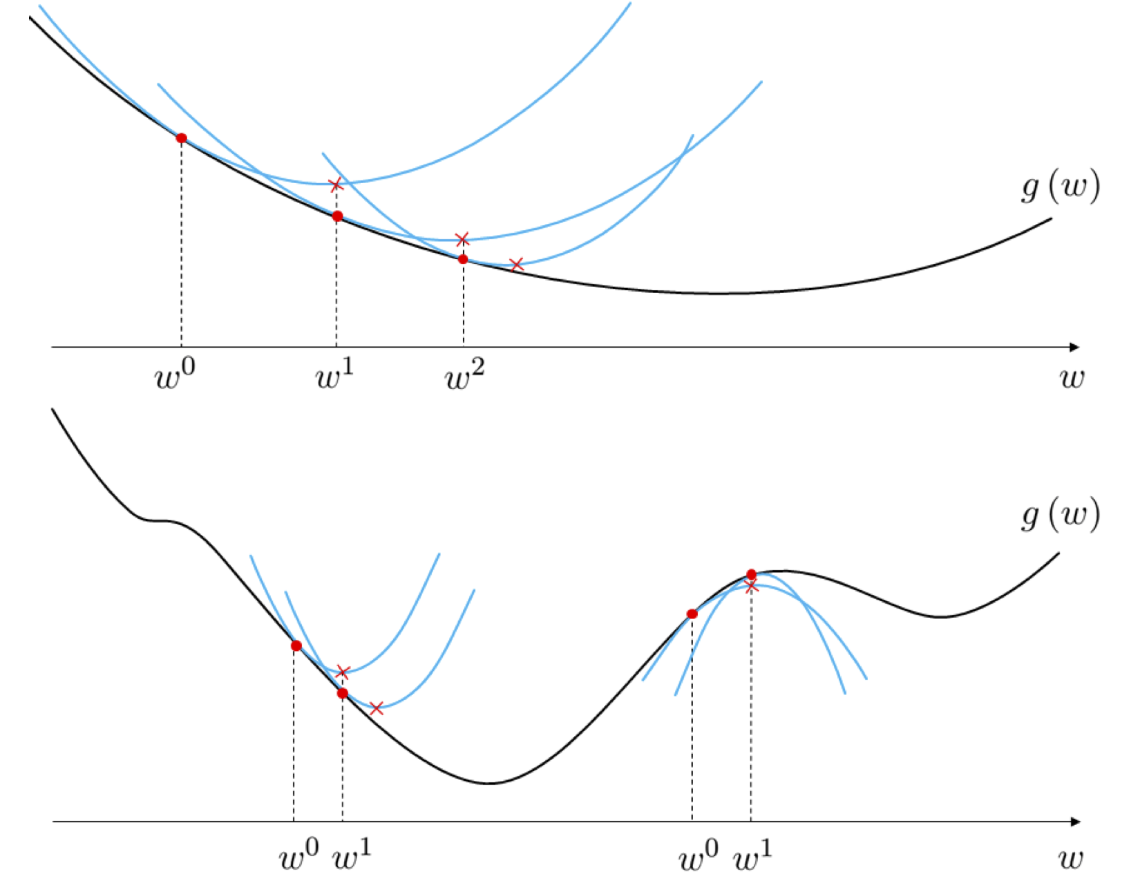
As illustrated in the top panel of Figure 1 - where these steps are drawn for a single-input function - starting at an initial point $\mathbf{w}^{0}$ Newton's method produces a sequence of points $\mathbf{w}^{1},\,\mathbf{w}^{2},\,...$ that minimize $g$ by repeatedly creating the second order Taylor series quadratic approximation to the function, and traveling to a stationary point of this quadratic. Because Newton's method uses quadratic as opposed to linear approximations at each step, with a quadratic more closely mimicking the associated function, it is often much more effective than gradient descent in the sense that it requires far fewer steps for convergence. However this reliance on quadratic information also makes Newton's method naturally more difficult to use with non-convex functions since at concave portions of such a function the algorithm can climb to a local maximum, as illustrated in the bottom panel of Figure 1, or oscillate out of control.
Note that although in the formula for the stationary point
\begin{equation} \mathbf{w}^{k} = \mathbf{w}^{k-1} - \left(\nabla^2 g(\mathbf{w}^{k-1})\right)^{-1}\nabla g(\mathbf{w}^{k-1}) \end{equation}
we invert the Hessian - an $N\times N$ matrix, where $N$ is the dimension of the input - in practice this is computationally expensive to implement. Instead $\mathbf{w}^k$ is typically found via solving the equivalent system of equations
\begin{equation} \nabla^2 g\left(\mathbf{w}^{k-1}\right)\mathbf{w} = \nabla^2 g\left(\mathbf{w}^{k-1}\right)\mathbf{w}^{k-1} - \nabla g(\mathbf{w}^{k-1}) \end{equation}
since this is a more efficient calculation. When more than one solution exists (e.g., if we are in a long narrow half-pipe of a convex function) the smallest possible solution is taken - this is typically referred to as the pseudo-inverse.
Take the single-input Newton step
\begin{equation} w^{k} = w^{k-1} - \frac{\frac{\mathrm{d}}{\mathrm{d}w}g(w^{k-1})}{\frac{\mathrm{d}^2}{\mathrm{d}w^2}g(w^{k-1})} \end{equation}
Near flat portions of a function both $\frac{\mathrm{d}}{\mathrm{d}w}g(w^{k-1})$ and $\frac{\mathrm{d}^2}{\mathrm{d}w^2}g(w^{k-1})$ are both nearly zero valued. This can cause serious numerical problems since once each (but especially the denominator) shrinks below machine precision the computer interprets $\frac{\frac{\mathrm{d}}{\mathrm{d}w}g(w^{k-1})}{\frac{\mathrm{d}^2}{\mathrm{d}w^2}g(w^{k-1})}\approx \frac{0}{0}$.
One simple and common way to avoid this potential disaster is to simply add a small positive value $\epsilon$ to the second derivative - either when it shrinks below a certain value or for all iterations. This regularized Newton's step looks like the following
\begin{equation} w^{k} = w^{k-1} - \frac{\frac{\mathrm{d}}{\mathrm{d}w}g(w^{k-1})}{\frac{\mathrm{d}^2}{\mathrm{d}w^2}g(w^{k-1}) + \epsilon} \end{equation}
The value of the regularization parameter $\epsilon$ is set by hand to a small positive value (e.g., $10^{-7}$). Note this is an adjustment made when the function being minimized is known to be convex, since in this case $\frac{\mathrm{d}^2}{\mathrm{d}w^2}g(w) \geq 0$ for all $w$.
The analogous adjustment for the multi-input case is to add $\epsilon \mathbf{I}_{N\times N}$ - a $N\times N$ identity matrix scaled by a small positive $\epsilon$ value - to the Hessian matrix. This gives the completely analogous regularized Newton's step for the multi-input case
\begin{equation} \mathbf{w}^{k} = \mathbf{w}^{k-1} - \left(\nabla^2 g(\mathbf{w}^{k-1}) + \epsilon \mathbf{I}_{N\times N}\right)^{-1}\nabla g(\mathbf{w}^{k-1}) \end{equation}
Note here that since again the function being minimized is assumed to be convex, adding this to the Hessian means that the matrix $\left(\nabla^2 g(\mathbf{w}^{k-1}) + \epsilon \mathbf{I}_{N\times N}\right)$ is always invertible. Nonetheless it is virtually always more numerically efficient to compute this update by solving the associated linear system $\left(\nabla^2 g(\mathbf{w}^{k-1}) + \epsilon \mathbf{I}_{N\times N}\right)\mathbf{w} = \left(\nabla^2 g(\mathbf{w}^{k-1}) + \epsilon \mathbf{I}_{N\times N}\right)\mathbf{w}^{k-1} - \nabla g(\mathbf{w}^{k-1})$ for $\mathbf{w}$.
This adjustment is so important and commonplace that we included it in both our formal pseudo-code and implementation below.
Note: while we used a maximum iterations convergence criterion is employed below, the the high computational cost of each Newton step often incentivizes the use of more formal convergence criterion (e.g., halting when the norm of the gradient falls below a pre-defined threshold). This also often incentivizes the inclusion of checkpoints that measure and/or adjust the progress of a Newton's method run in order to avoid problems near flat areas of a function.
1: input: function $g$, maximum number of steps $K$, initial point $\mathbf{w}^0$, and regularization parameter $\epsilon$
2: for $k=1...K$
3: $\mathbf{w}^{k} = \mathbf{w}^{k-1} - \left(\nabla^2 g(\mathbf{w}^{k-1}) + \epsilon \mathbf{I}_{N\times N}\right)^{-1}\nabla g(\mathbf{w}^{k-1})$
4: output: history of weights $\left\{\mathbf{w}^{k}\right\}_{k=0}^K$ and corresponding function evaluations $\left\{g\left(\mathbf{w}^{k}\right)\right\}_{k=0}^K$
# using an automatic differentiator - like the one imported via the statement below - makes coding up gradient descent a breeze
from autograd import grad
from autograd import hessian

# newtons method function - inputs: g (input function), max_its (maximum number of iterations), w (initialization)
def newtons_method(g,max_its,w,**kwargs):
    # compute gradient module using autograd
    gradient = grad(g)
    hess = hessian(g)

    # set numericxal stability parameter / regularization parameter
    epsilon = 10**(-7)
    if 'epsilon' in kwargs:
        beta = kwargs['epsilon']

    # run the newtons method loop
    weight_history = [w]           # container for weight history
    cost_history = [g(w)]          # container for corresponding cost function history
    for k in range(max_its):
        # evaluate the gradient and hessian
        grad_eval = gradient(w)
        hess_eval = hess(w)

        # reshape hessian to square matrix for numpy linalg functionality
        hess_eval.shape = (int((np.size(hess_eval))**(0.5)),int((np.size(hess_eval))**(0.5)))

        # solve second order system system for weight update
        A = hess_eval + epsilon*np.eye(w.size)
        b = grad_eval
        w = np.linalg.solve(A,np.dot(A,w) - b)

        # record weight and cost
        weight_history.append(w)
        cost_history.append(g(w))
    return weight_history,cost_history
In the next Python cell we animate the process of performing Newton's method to minimize the function
\begin{equation} g(w) = \frac{1}{50}\left(w^4 + w^2 + 10w \right) + 0.5 \end{equation}
beginning at the point $w = 2.5$ marked as a magenta dot (and corresponding evaluation of the function marked as magenta X).
Moving the slider from left to right animates each step of the process in stages - the second order approximation is shown in light blue, then its minimum is marked with a magenta dot on the input space, along with the evaluation on the quadratic and function $g$ marked as a magenta and blue X respectively. As Newton's method continues each step is colored from green - when the method begins - to red as it reaches the maximum number of pre-defined iterations (set here to 5).
# load video into notebook
from IPython.display import HTML
HTML("""
<video width="1000" height="400" controls loop>
  <source src="videos/animation_8.mp4" type="video/mp4">
  </video>
""")
Below we apply a single Newton step to completely minimize the quadratic function
\begin{equation} g(w_1,w_2) = 0.26(w_1^2 + w_2^2) - 0.48w_1w_2 \end{equation}
This can be done with a single step because the second order Taylor series - being a quadratic (local) approximation to a function - of a quadratic function is simply itself, and thus reduces to solving the first order system of a quadratic function (a linear system of equations). We compare a run of $100$ steps of gradient descent (left panel) with a single Newton step (right panel).

Indeed this is the same solution identified visually in the plot above.
While we have seen in the derivation of Newton's method that - being a local optimization approach - it does have an steplength parameter $\alpha$ it is implicitly set to $\alpha = 1$ and so appears 'invisible'. However note that one can explicitly introduce a steplength parameter $\alpha$ and - in principle - use adjustable methods, e.g., backtracking line search (described the previous Chapter in the context of gradient descent) in order to tune $\alpha$. Adding a steplength parameter $\alpha$ this explicitly weighted Newton step looks like
\begin{equation} \mathbf{w}^{k} = \mathbf{w}^{k-1} - \alpha\left(\nabla^2 g(\mathbf{w}^{k-1})\right)^{-1}\nabla g(\mathbf{w}^{k-1}) \end{equation}
with the standard Newton's method step falling out when $\alpha = 1$.