code

share


As we discussed in detail in Section 11.4, validation data is the portion of our original dataset we exclude at random from the training process in order to determine a proper tuned model that will faithfully represent the phenomenon generating our data. The validation error generated by our tuned model on this 'unseen' portion of data is the fundamental measurement tool we use to determine an appropriate cross-validated model for our entire dataset (besides, perhaps, a testing set - see Section 11.7). However, the random nature of splitting data into training and validation poses a potentially an obvious flaw to our cross-validation process: what if the random splitting creates training and validation portions which are not desirable representatives of the underlying phenomenon that generated them? In other words, in practice what do we do about potentially bad training-validation splits, which can result in poorly representative cross-validated models?
Because we need cross-validation in order to choose appropriate models in general, and because we can do nothing about the (random) nature by which we split our data for cross-validation (what better is there to simulate the 'future' of our phenomenon?), the practical solution to this fundamental problem is to simply perform several different training-validation splits, determine an appropriate cross-validated model on each split, and then average the resulting cross-validated models. By averaging a set of cross-validated models, also referred to as bagging in the jargon of machine learning, we can very often both 'average out' the potentially undesirable characteristics of each model while synergizing their positive attributes (that is, while bagging is not mathematically guaranteed to produce a more effective model than any of the members averaged to create it - e.g., when all but one cross-validated model provide poor results leading to an average of mostly bad predictors - typically in practice it produces superior results). Moreover, with bagging we can also effectively combine cross-validated models built from different universal approximators. Indeed this is the most reasonable way of creating a single model built from different types of universal approximators in practice.
Here we will walk through the concept of bagging or model averaging for regression, as well as two-class and multi-class classification by exploring an array of simple examples. With these simple examples we will illustrate the superior performance of bagged models visually, but in general we confirm this using the notion of testing error (see Section 11.7) or an estimate of testing error (often employed when bagging trees - see Section 14.6). Regardless, the principles detailed here can be employed more widely as well to any machine learning problem. As we will see, the best way to average/bag a set of cross-validated regression models is by taking their median and cross-validated classification models by computing the mode of their predicted labels.
Here we explore several ways of bagging a set of cross-validated models for simple nonlinear regression dataset. As we will see, more often than not the best way to bag (or average) cross-validated regression models is by taking their median (as opposed to their mean).
In the set of small panels in the left side of Figure 11.47 we show $10$ different training-validation splits of a prototypical nonlinear regression dataset, where $\frac{4}{5}$ of the data in each instance has been used for training (colored light blue) and $\frac{1}{5}$ is used for validation (colored yellow). Plotted with each split of the original data is the corresponding cross-validated spanning set model found by naively cross-validating (see Section 11.4) the range of complete polynomial models of degree $1$ to $20$. As we can see, while many of these cross-validated models perform quite well, several of them (due to the particular training-validation split on which they are based) severely underfit or overfit the original dataset. In each instance the poor performance is completely due to the particular underlying (random) training-validation split, which leads cross-validation to a validation error minimizing tuned model that still does not represent the true underlying phenomenon very well. By taking an average (here the median) of the $10$ cross-validated models shown in these small panels we can average-out the poor performance of this handful of bad models, leading to a final bagged model that fits the data quite well - as shown in the large right panel of Figure 11.47.
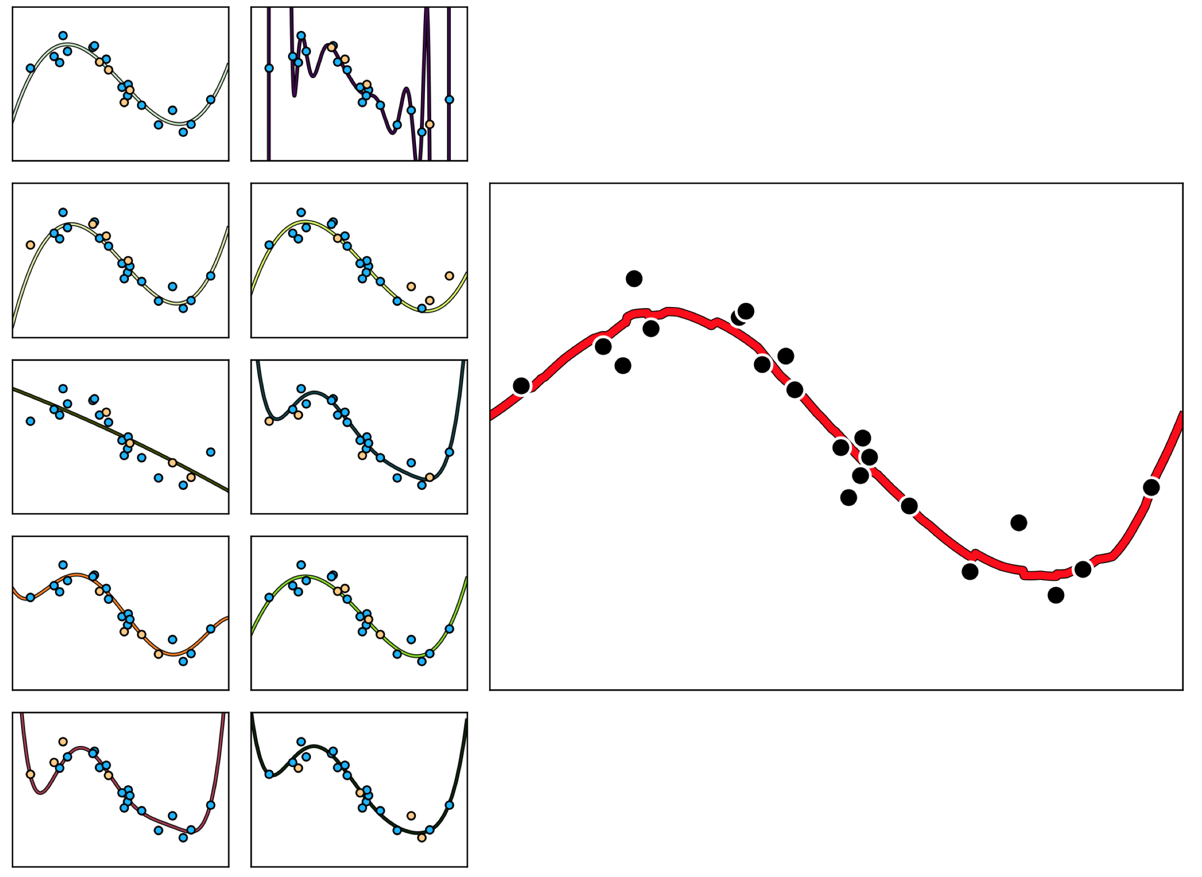
More generally, if we created $E$ cross-validated regression models $\left\{\text{model}_{e}\left(\mathbf{x},\Theta_e^{\star}\right)\right\}_{e=1}^E$, each trained on a different training-validation split of the data, then our median model $\text{model}\left(\mathbf{x},\Theta\right)$ as
\begin{equation} \text{model}\left(\mathbf{x},\Theta^{\star} \right) = \text{median}\left\{ \text{model}_{e}\left(\mathbf{x},\Theta_e^{\star}\right)\right\}_{e=1}^E. \end{equation}
Note here the parameter set $\Theta^{\star}$ of the median model contains all of tuned parameters $\left\{\Theta_e^{\star}\right\}_{e=1}^E$ from the models in cross-validated set.
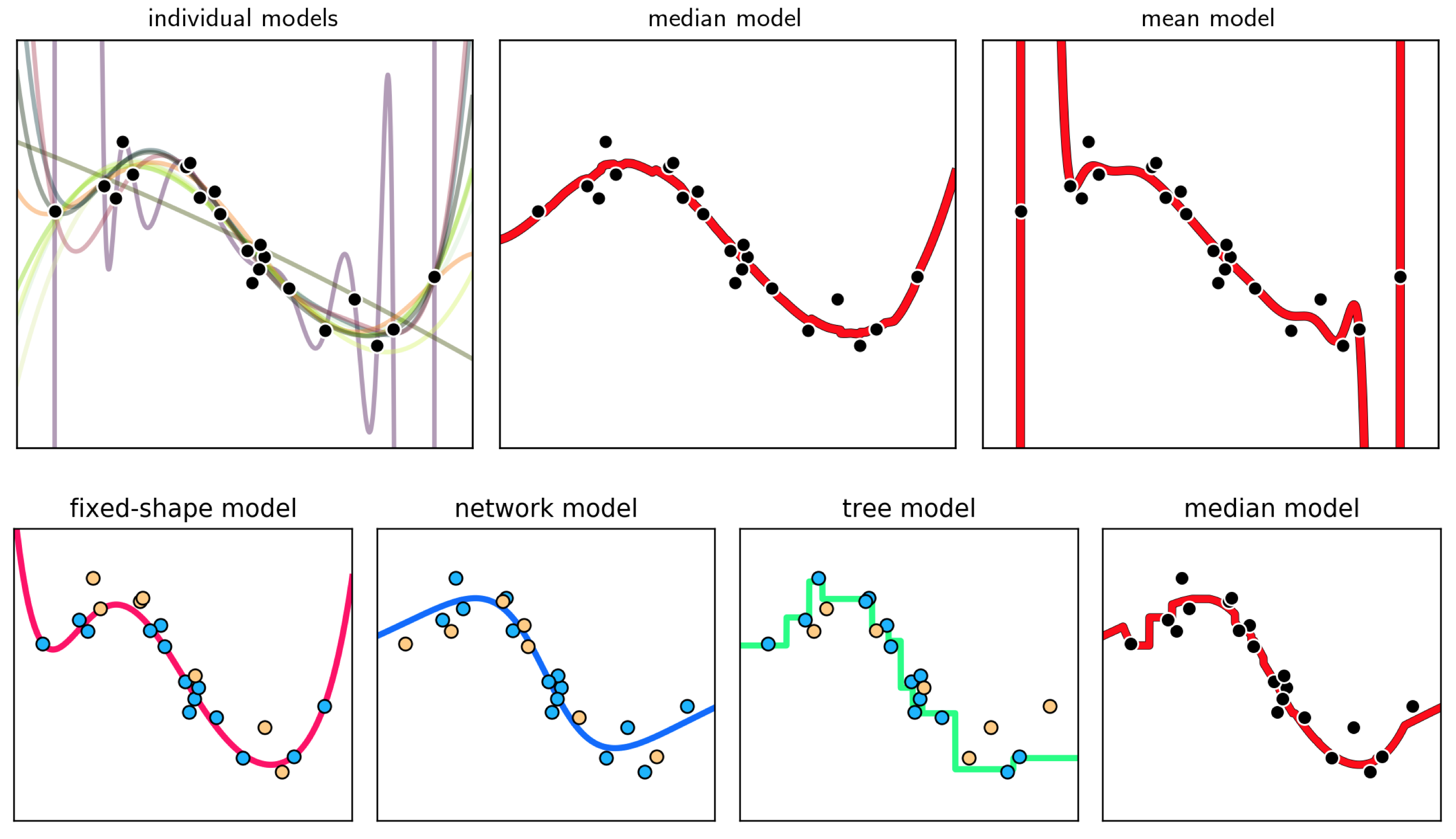
Why average our cross-validated models using the median as opposed to say the mean? Because the mean of a long list of numbers is far more sensitive to outliers than is the median. In using the median of a large set of cross-validated models - and thus by using the median of their corresponding fits to the entire dataset - we ameliorate the effect of severely underfitting / overfitting cross-validated model on our final bagged model. In the top row of Figure 48 we show the regression dataset shown previously along with the individual cross-validated fits (left panel), the median bagged model (middle panel), and the mean bagged model (right panel). Here the mean model is highly affected by the few overfitting models in the group, and ends up being far too oscillatory to fairly represent the phenomenon underlying the data. The median is not affected in this way, and is a much better representative.
When we bag we are simply averaging various cross-validated models with the desire to both avoid bad aspects of poorly performing models, and jointly leverage strong elements of the well performing ones. Nothing in this notion prevents us from bagging together cross-validated models built using different universal approximators, and indeed this is the most organized way of combining different types of universal approximators in practice.
In the bottom row of Figure 11.48 we show the result of a cross-validated polynomial model (left panel) built by naively cross-validating full polynomials of degree $1$ through $10$, a naively cross-validated (see Section 11.4) neural network model (in the second to the left panel) built by comparing models consisting of $1$ through $10$ units, and a cross-validated stump model (second to the right panel) built via boosting (see Section 11.5). Each cross-validated model uses a different training-validation split of the original dataset, and the bagged (median) of these models is shown in the right panel.
The principle behind bagging cross-validated models holds analogously for classification tasks, just as it does with regression. Because we cannot be certain whether or not a certain (randomly chosen) validation set accurately represents the 'future data' from a given phenomenon well, the averaging (or bagging) of a number of cross-validated classification models provides a way of 'averaging out' poorly representative portions of some models while combining the various models' positive characteristics.
Because the predicted output of a (cross-validated) classification model is a discrete label via, e.g., passing the model through the $\text{sign}$ function in the case of two-class classification (when employing label values $y\in\left\{-1,+1\right\}$ as detailed in Chapter 6) or the fusion rule in the multi-class setting (as detailed in Chapter 7) the average used to bag cross-validated classification models is the mode (i.e., the most popularly predicted label).
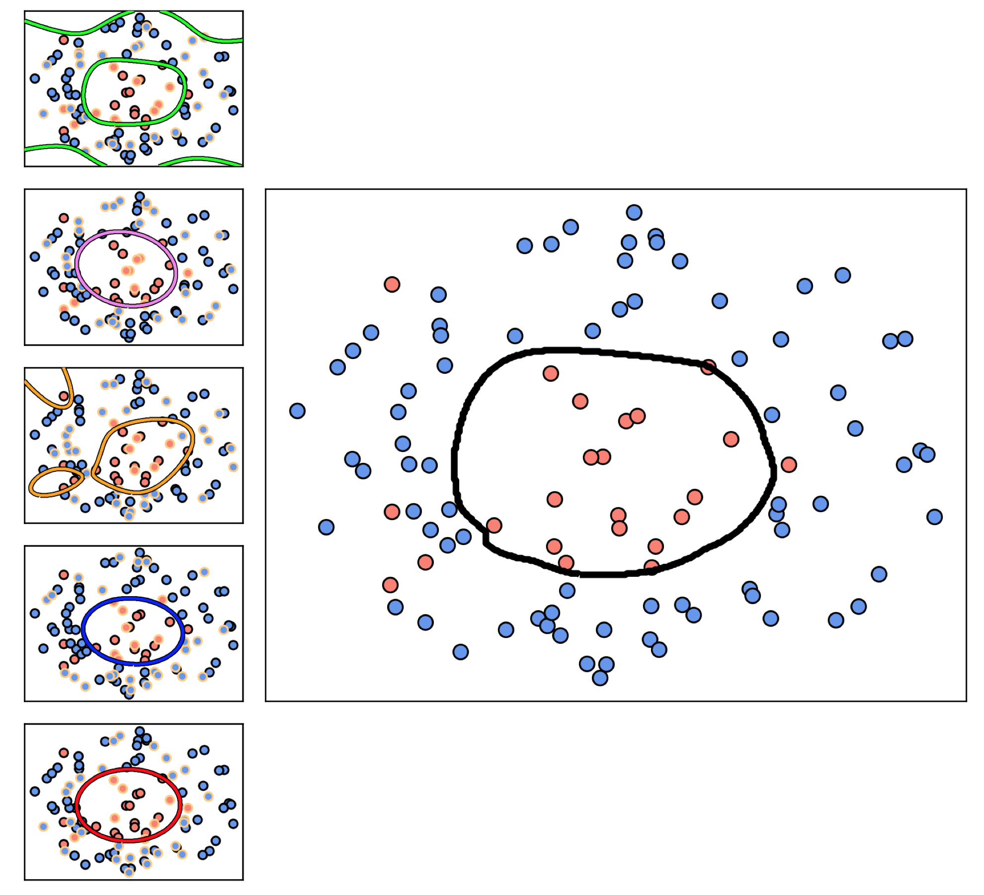
In the set of small panels in the left column of Figure 11.49 we show $5$ different training-validation splits of the prototypical two-class classification dataset, where $\frac{2}{3}$ of the data in each instance is used for training and $\frac{1}{3}$ is used for validation (the edges of these points are colored yellow). Plotted with each split of the original data is the nonlinear decision boundary corresponding to each cross-validated model found by naively cross-validating the range of complete polynomial models of degree $1$ to $8$. Many of these cross-validated models perform quite well, but several of them (due to the particular training-validation split on which they are based) severely overfit the original dataset. By bagging these models using the most popular prediction to assign labels (i.e., the mode of these cross-validated model predictions) we produce an appropriate decision boundary for the data shown in the right panel of the Figure.
In the top-middle panel of Figure 11.50 we illustrate the decision boundary from each of $5$ naively cross-validated models each built using $B = 20$ single layer $\text{tanh}$ units trained on different training / validation splits of the dataset shown in the top-left panel of the Figure. In each instance $\frac{1}{3}$ of the dataset is randomly chosen as validation (and is highlighted in yellow), and the appropriate tuning of each model's parameters is achieved via $\ell_2$ regularization based cross-validation (see Section 11.6) using a dense range of values for $\lambda \in [0,0.1]$. In the top-middle panel we plot the diverse set of decision boundaries associated to each cross-validated model on top of the original dataset, each colored differently so they can be distinguished visually. While some of these decision boundaries separate the two classes quite well, others do a poorer job. In the top-right panel we show the decision boundary of the bag, created by taking the mode of the predictions from these cross-validated models, which performs quite well.
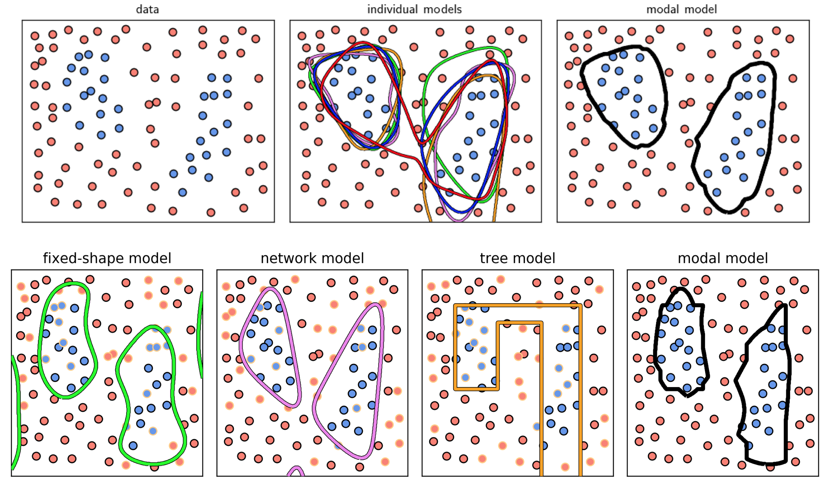
As with regression, with classification we can also combine cross-validated models built from different universal approximators. We illustrate this in the bottom row of Figure 11.50 using the same dataset. In particular we show the result of a naively cross-validated polynomial model (left panel) built by comparing full polynomials of degree $1$ through $10$, a naively cross-validated neural network model (in the second to the left panel) built by comparing models consisting of $1$ through $10$ units, and a cross-validated stump model (second to the right panel) built via boosting over a range of $20$ units. Each cross-validated model uses a different training-validation split of the original dataset (the validation data portion highlighted in yellow in each panel), and the bag (mode) of these models shown in the right panel performs quite well.
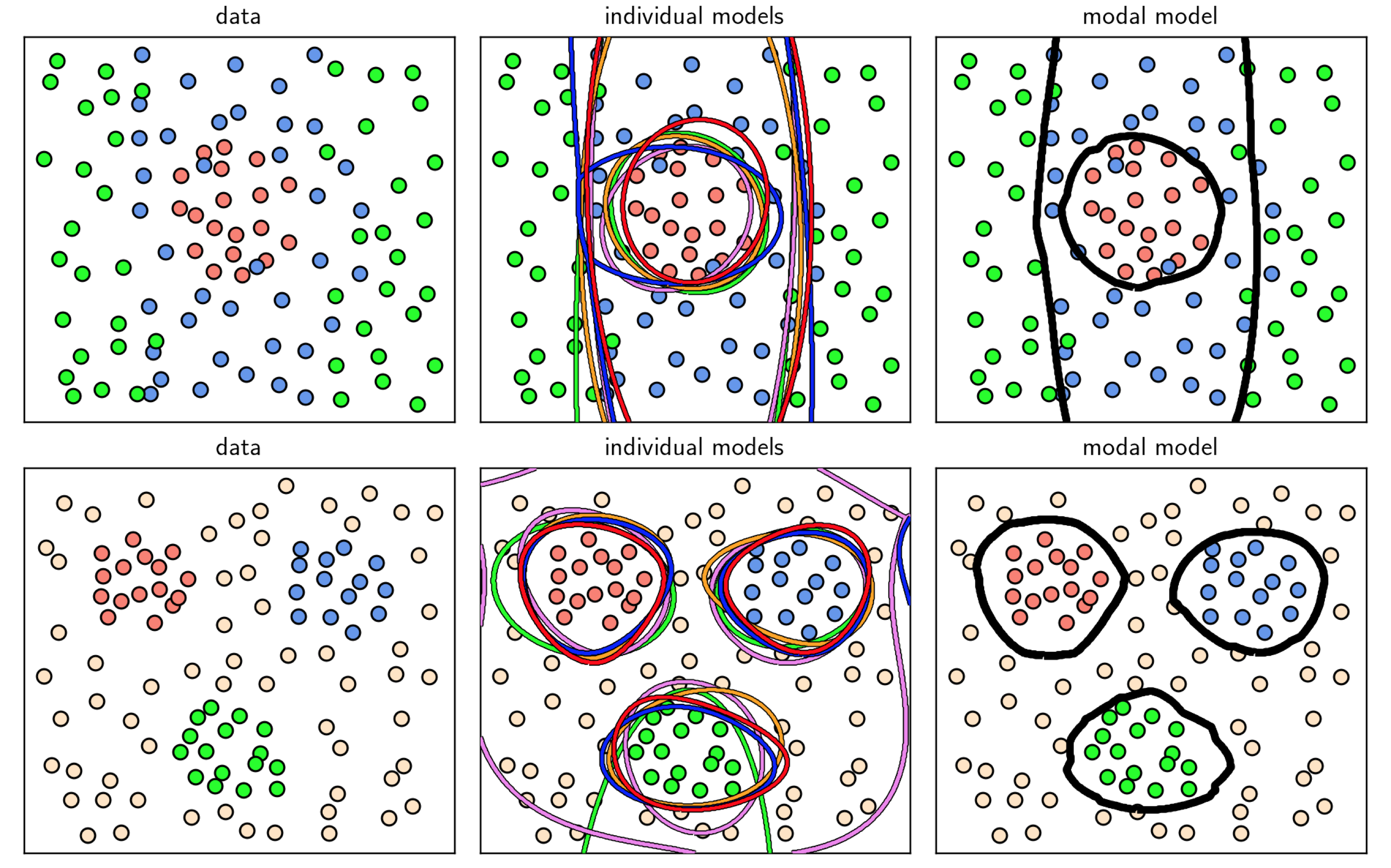
In this example we illustrate the bagging of various cross-validated multi-class models on two different datasets, shown in the left column of Figure 11.51. In each case we naively cross-validate full polynomial models of degree $1$ through $5$, with $5$ cross-validated models learned in total. In the middle column of the Figure we show the decision boundaries provided by each cross-validated model in distinct colors, while the decision boundary of the final modal model is shown in the right column for each dataset, which perform very well.
Note that in the Examples of this Section the exact number of cross-validated models bagged were set somewhat arbitrarily. Like other important parameters involved with cross-validation (e.g., the portion of a dataset to reserve for validation) there is in general no magic number (of cross-validated models) used generally in practice for bagging. Ideally if we knew that any random validation portion of a dataset generally represented it well, which is often true with very large datasets, there would be less of a need to ensemble multiple cross-validated models where each was trained on a different training/validation split of the original data, since we could trust the results of a single cross-validated model more. Indeed in such instances we could instead bag a range of models trained on a single training/validation split in order to achieve similar improvements over a single model. On the other hand, the less we could trust in the faithfulness of a random validation portion to represents a phenomenon at large, the less we could trust an individual cross-validated model and hence we might wish to ensemble more of them to help average our poorly performing models resulting from bad splits of the data. Since this is generally impossible to determine in practice often practical considerations (e.g., computation power, dataset size) determine if bagging is used and if so how many models are employed in the average.
The bagging technique described here, wherein we combine a number of different models each cross-validated independently of the others, is a primary example of what is referred to as ensembling in the jargon of machine learning. An ensembling method (as the name ‘ensemble’ implies) generally refers to any method of combining different models in a machine learning context. Bagging certainly falls into this general category, as does the general boosting approach to cross-validation described in Section 11.5. However, these two ensembling methods are very different from one another.
With boosting we build up a single cross-validated model by gradually adding together simple models consisting of a single universal approximator unit. Each of the constituent models involved in boosting are trained in a way that makes each individual model dependent on its predecessors (who are trained first). On the other hand with bagging (as we have seen) we average together multiple cross-validated models that have been trained independently of each other. Indeed any one of those cross-validated models in a bagged ensemble can itself be a boosted model.