code

share


In this Section we detail a twist on the notion of ensembling called K-fold cross-validation, that is often applied when human interpret-ability of a final model is of significant importance. While ensembling often provides a better fitting averaged predictor that avoids the potential pitfalls of any individual cross-validated model, human interpret-ability is typically lost as the final model is an average of many potentially very different nonlinearities (stumps / tree-based approximators are sometimes an exception to this general rule, as detailed in Section 14.1). Instead of averaging a set of cross-validated models over many splits of the data, each of which provides minimum validation error over a respective split, with K-folds cross-validation we choose a single model that has minimum average validation error over all splits of the data. This produces a potentially less accurate final model, but one that is significantly simpler (than an ensembled model) and can be more easily understood by humans. As we will see, in special applications K-folds is also used with linear models as well.
K-folds cross-validation is a method for determining robust cross-validated models via an ensembling-like procedure that constrains the complexity of the final model so that it is more human-interpretable. Instead of averaging a group of cross-validated models, each of which achieves a minimum validation over over a random training-validation split of the data, with K-folds cross-validation we choose a single final model that achieves the lowest average validation error over all of the splits together. By selecting a \emph{single model} to represent the entire dataset, as opposed to an average of different models as is done with ensembling, we make it easier to human-interpret the selected model.
Of course the desire for any nonlinear model to be interpretable means that its fundamental building blocks (universal approximators of a certain type) need to be interpretable as well. Neural networks, for example, are almost never human interpretable while fixed-shape (most commonly polynomials) and tree-based approximators (commonly stumps) can be interpreted depending on the problem at hand. Thus the latter two types of universal approximators are more commonly employed with the K-folds technique.
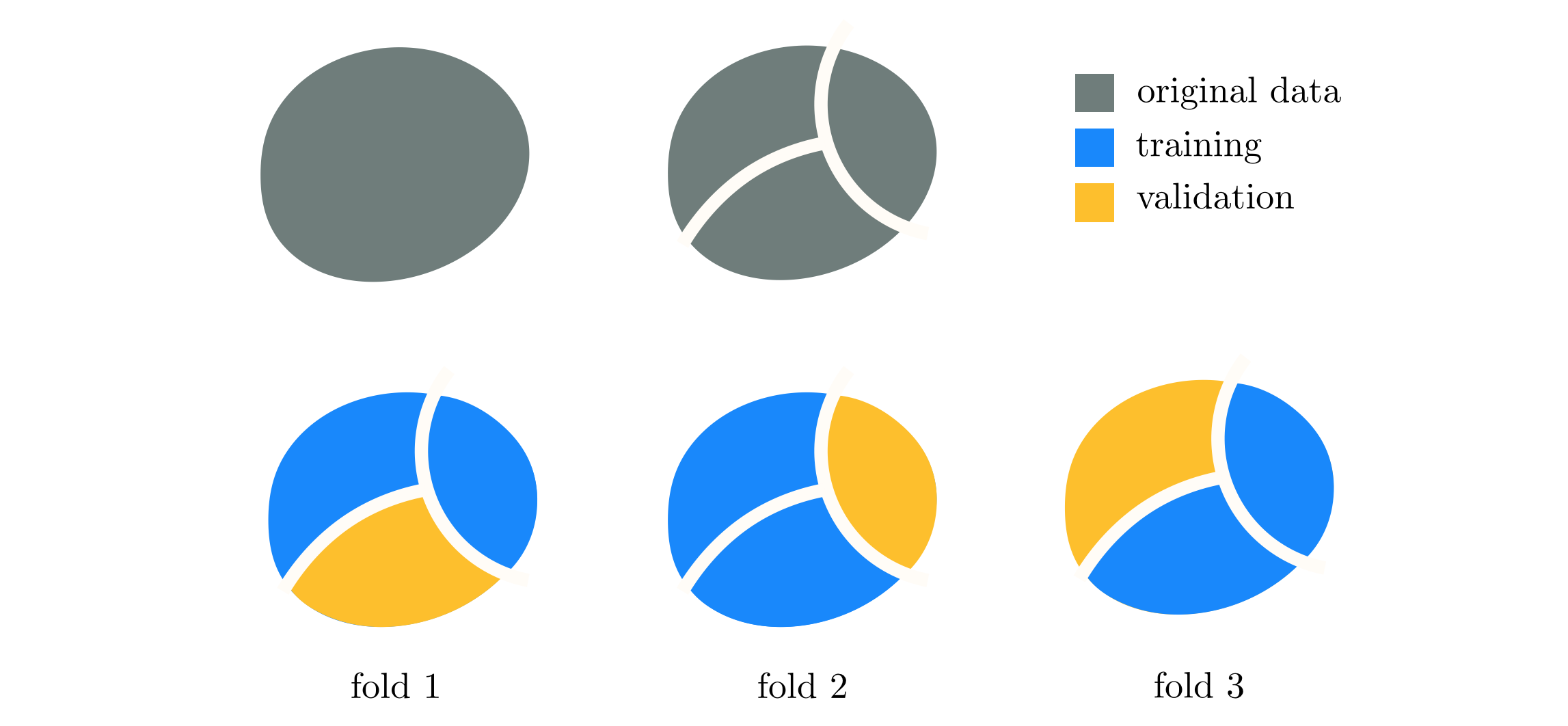
To further simplify the final outcome of this procedure instead of using completely random training-validation splits, as done with ensembling, we split the data randomly into a set of $K$ non-overlapping pieces. This is depicted visually in Figure 11.52, where the original data is represented as the entire circular mass (top left panel) is split into $K=3$ non-overlapping sets (bottom row). We then cycle through $K$ training-validation splits of the data that consist of $K-1$ of these pieces as training, with the final portion as validation, which allows for each point in the dataset to belong to a validation set precisely one time. Each such split is referred to as a fold, of which there are $K$ in total, hence the name 'K-folds.' On each fold we cross-validate the same set of models and record the validation score of each. Afterwards we choose the single best model that produced the lowest average validation error. Once this is done the minimum average validation model is re-trained over the entire dataset to provide a final tuned predictor of the data.
Since no models are combined / averaged together with K-folds, it can very easily produce less accurate models (in terms of testing error - see Section 11.7) for general learning problems when compared to ensembling. However, when human interpret-ability of a model overshadows the needs for exceptional performance, K-folds produces a stronger performing model than a single cross-validated model that can still be understood by human beings. This is somewhat analogous to the story of feature selection detailed in Sections 11.5 and 11.6, where human interpret-ability is the guiding motivator (and not simply model effectiveness). In fact the notion of feature selection and K-folds cross-validation indeed intersect in certain applications, one of which we will see in the Examples below.
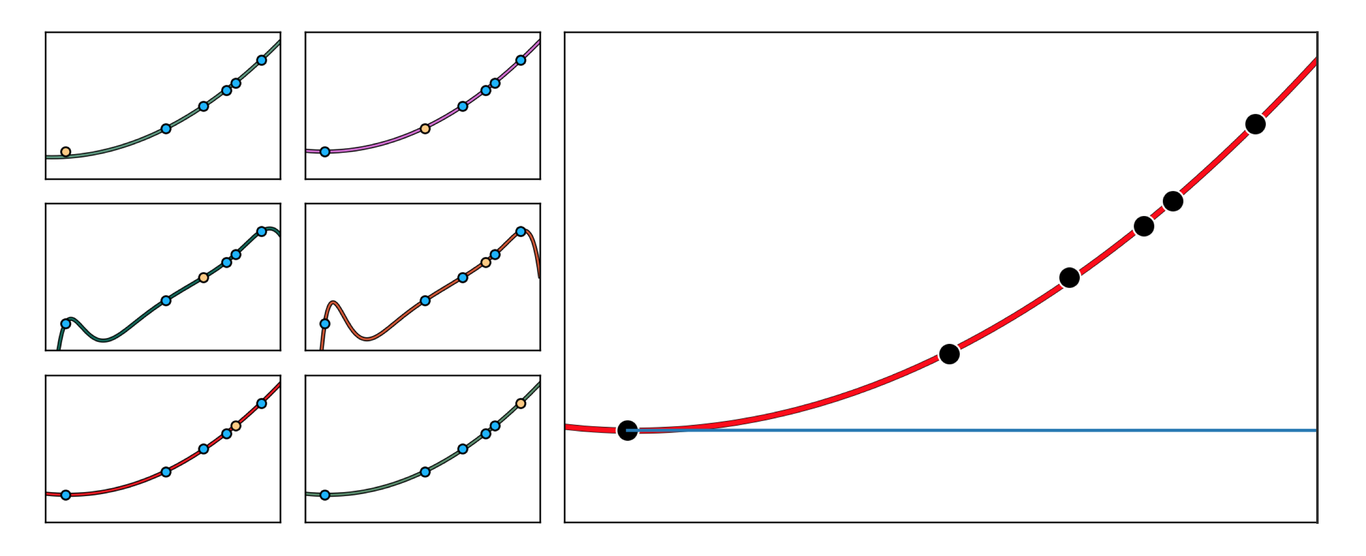
In this Example we use K-folds cross-validation on the Galileo dataset detailed in Example 3 of Section 10.2 to recover the quadratic rule that was both engineered there, and that Galileo himself divined from a similar dataset. In the left column of Figure 11.53 we show how using $K=P$ fold cross-validation (since we have only $P=6$ data points intuition suggests, that we use a large value for $K$ as described in Section 11.4), sometimes referred to as leave-one-out K-folds cross -validation, allows us to recover precisely the quadratic fit Galileo made by eye. Note that by choosing $K=P$ this means that every data point will take a turn being the testing set. Here we search over the polynomial models of degree $M=1,...,6$ since they are not only interpretable, but are appropriate for data gleaned from physical experiments (which often trace out smooth rules). While not all of the models over the $6$ folds fit the data well, the average K-folds result is indeed the $M^{\star}=2$ quadratic polynomial fit originally proposed by Galileo.
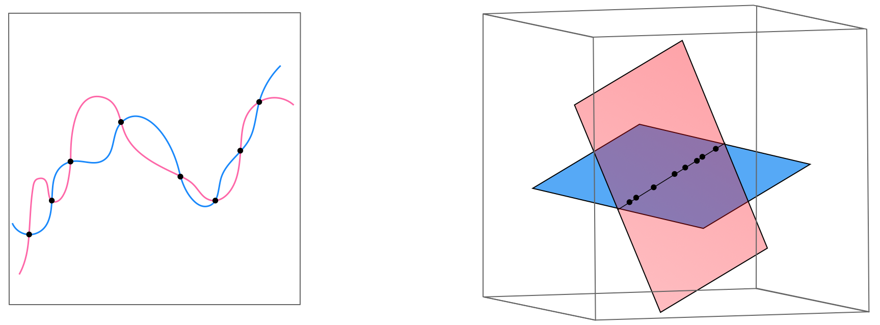
Suppose for a moment we have a high capacity model which enables several kinds of overfitting behavior for a nonlinear regression dataset, with each overfitting instance of the model provided by different settings of the linear combination weights of the model (suppose any internal parameters of its features are fixed). We illustrate such a scenario in the left panel of Figure 11.54, where two settings of such a model provide two distinct overfitting predictors for a generic nonlinear regression dataset. As we learned in Section 10.2, any nonlinear model in the original space of a regression dataset corresponds to a \emph{linear model} in the transformed feature space (i.e., the space where each individual input axis is given by one of the chosen nonlinear feature). Since our model easily overfits the original data, in the transformed feature space our data lies along a linear subspace that can be perfectly fit using many different hyperplanes. Indeed the two nonlinear overfitting models shown in the left panel of the Figure correspond one-to-one with the two linear fits in the transformed feature space - here illustrated symbolically in the right panel of the Figure (in reality we could not visualize this space, as it would likely be too high dimensional). In other words, a severely overfitting high capacity \emph{nonlinear model} in the original regression space is severely overfitting high capacity linear model in the transformed feature space feature. This fact holds regardless of the problem type.
The general scenario detailed in the right panel of Figure 11.54 is precisely where we begin when faced with small datasets that have very high input dimension: in such scenarios \emph{even a linear model has extremely high capacity and can easily overfit}, virtually ruling out the use of more complicated nonlinear models. Thus in such scenarios, in order to properly tune the parameters of a high capacity (linear) model we often turn to the cross-validation technique designed specifically to block high capacity models: regularizer-based regularization (as described in Section 11.6). Given the small amount of data at play to determine the best setting of the regularization parameter K-folds is commonly employed to determine the proper regluarization parameter value and ultimately the parameters of the linear model.
This scenario often provides an interesting point of intersection with the notion of feature selection via regularization detailed in Section 9.7. Employing the $\ell_1$ regularizer we can block the capacity of our high capacity linear model while simultaneously selecting important input features, making human interpret-ability possible.
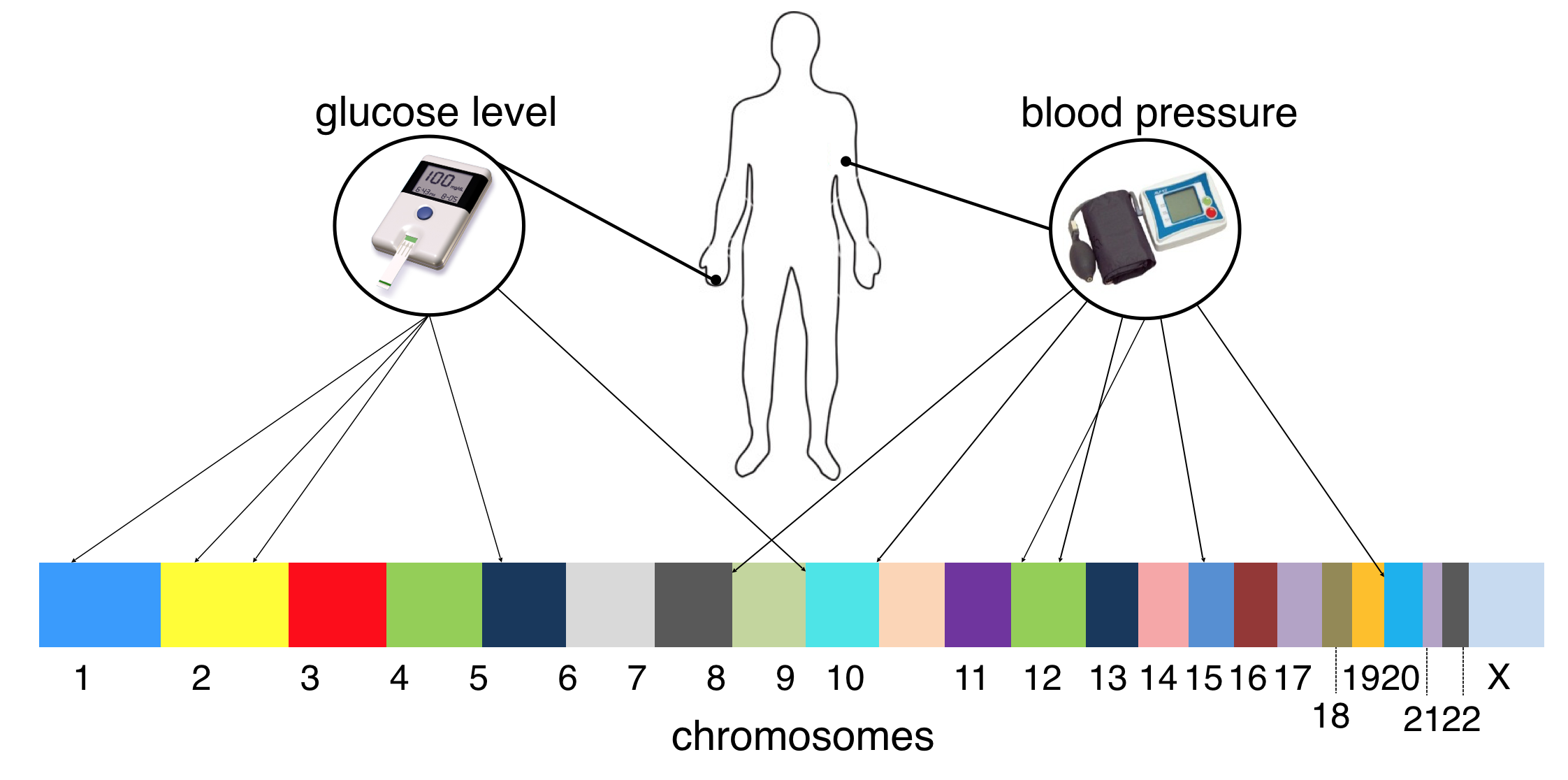
Genome-wide association studies (GWAS) aim at understanding the connections between tens of thousands of genetic markers, taken from across the human genome of several subjects, with diseases like high blood pressure and cholesterol, heart disease, diabetes, various forms of cancer, and many others. These studies typically produce small datasets of high dimensional (input) genetic information taken from a sample of patients with a given affliction and a control group of non-afflicted (see Figure 11.55). Thus regularization based cross-validation a useful tool for learning meaningful (linear) models for such data. Moreover using a feature selecting regularizer like the $\ell_1$ norm can help researchers identify the handful of genes critical to affliction, which can both improve our understanding of disease and perhaps provoke development of gene-targeted therapies.